Optimal Stopping in Sampling from a Bivariate Distribution

Vol. 16, No. 3, September 1973.

OPTIMAL STOPPING IN SAMPLING FROM

A BIVARIATE DISTRIBUTION

MINORU SAKAGUCHI Osaka University

(Received September 18, 1972) Abstract

This paper studies an optimal stopping problem without recall in which the experimenter observes a sequential random sample from a specified bivariate probability distribution. The problem can be interpreted as deciding to buy a house which has the two-dimensional worth, for example, the values for a husband and for his wife. The concept of equilibrium neutral values is introduced, and by using it the explicit solutions are derived for the infinite-opportunity case and for the finite case. The examples are included to illustrate the com-putations required by the "optimal" strategy_

1. Introduction

Let (Xi, Yi), i== I, 2, ... , be independent and identically distributed bivariate random variables that can be observed sequentially at a cost of Cl and C2 (both~O) per observation of X and Y, respectively. The common distribution function H(x, y) of each of the observation (Xi, Yi) is assumed to be known to the observer which we shall here-after call the experimenter. We shall suppose that if the experimenter terminates the sampling process after having observed the values (Xi=Xi, Yi=Yi), i=:l, ... , rn, his gain is a pair of values xm-rnCl and

Ym-mC2. We are now interested in finding a stopping rule which can be considered as optimal in some reasonable sense. This formu-lation of the problem provides a model for studying an immediate extension of optimal stopping problems, exhaustively discussed in [1]. For the sake of a concrete example, consider a man who desires to buy a house. There is a large population of houses available, and he proceeds by selecting one of these at random and going to see it. Having done this, he may either reject it immediately as being un-satisfactory and go on to look at another, or he may buy it on the spot, which has the eventual outcome of the two-dimensional reward eX, Y). We may consider, for example, X as representing monetary worth of the house, and Yas representing travelling expenses from the location of the house to his working place. We may also consider X and Y as the values of the house for him, and for his wife, respectively.

We shall suppose that there is a given upper bound n, 2;2;n;2;00,

on the number of observations that can be taken. Since the sequen-tial sampling is taken from a bivariate distribution we shall introduce the concept of equilibrium neutral values, and by using it the explicit solutions are derived for the case where Cl, C2>O and n=oo in Section 2, and the case where Cl=C2=O and /1,<00 in Section 3. In the final section some examples are given in order to illustrate the computa-tions required by the" optimal" strategy.

2. Optimal Strategy for the Case Where the Number of Observations is not Limited

We shall consider a class of stopping rules in which the experi-menter has a pair of "neutral" values u and v such that, the sampling procedure is terminated at the first in such that Xm~U and Ym::2:V.

Let !"=!"(u, v) denote the random stopping time when the neutral values u and v are used. Let

(1) fM1(u, v)=E[X,-TCllu, V], (M2(U, v)=E( Y,-TC21 u, V] •

Then Ml(U, v) is the expected net gain from the observations of X when using the neutral values (u, v). M2(U, v) has the similar meaning. Now the experimenter wants to maximize his expected net gains of both X and Y. In such cases the concept of the equilibrium points in the context of non-cooperative game theory [5] would be useful. Under this concept the neutral value Tt is chosen so as to try to

maximize the net gain Ml(U, v), and simultaneously the value of v to maximize M2(U, v). An equilibrium point (u*, v*) for the functions Ml(U, v) and M2(U, v) is a pair of values u* and v* such that each value maximizes its own net gain if the other value is held fixed. More precisely,

{

Ml(U*' v*)=~ax M1(u, v*) ,

(2 )

M2(U*, v*)=maxM2(u*, v) .

v

Continuing to work within the framework of net-gains maximiza-tion, we recognize that if we partially differentiate expressions for Ml(U, v) and M2(U, v) with respect to U and v respectively, equate the partial derivatives to zero and solve the resultant equations then we shall obtain the equilibrium pair of values. We prove!):

Theorem 1:

(i) Let S denote the event {X~u, ~v}. Then we have

(3) fM1(u, v)=E[XI S]-cl/Pr{S} (M2(U, v)=E[YI S]-c2/Pr{S},

where E['I

SI

denotes the conditional expectation under the condition that the event S has occurred.

( ii ) The equilibrium point (u*, v*) satisfies the simultaneous

1) This paper was motivated by an article by Matsuda and Sekiguchi [4].

equations (4) {E[X-U

I

S]=cljPr{S} E[Y-vl S]=c2jPr{S}. Moreover we have { Ml(U*, v*)

=

U* (5 ) M2(U*, v*)=v* . =

Proof. (i): Ml(U, v)=E[X,-rcd=

2::,

(l-Pr{S})m-1 Pr{S}E[X-mcll SJ

m-=l

[E[XI S] Cl ]

=Pr{S} Pr{S} (Pr{S})2 =E[XI S]-cljPr{S} , and similarly for M2(U, v).

( ii) Suppose the cumulative distribution function (ab. by cdf)

H(x, y) has the probability density function (abbr. by pdf) hex, y). Then from (3) ( 3') [

XdX~~ h(x~,

y)dy-c! [dX

~~h(a:,

y)dy

~=YdY~=

h(:r., y)dX-C2 M₂(u v)= v u _ _ _ _ _ , _{[dY [h(:r, y)dx}

C arrymg t roug t e computatlOns . h h h . --au aM! =--av-= aM2 0 we 0 b · tam

(4')

~:(X-U)dX~~

hex, y)dy=:c!,

~~(Y-V)dY[

hex, y)dX=C2

which is equivalent to (4). (3), combined with (4) and taking (u, v)= (u*, v*), give (5), completing the proof.

For later use we shall rewrite the expressions (4) or (4') in two different ways as follows: Let

F[~v]=conditional cdf of X given that ~v G[X~u]=conditional cdf of Y given that X~u .

For any cdf K(z) of the random variable Z with finite mean

[00

zdK(z),

define

Tx(t) =

~~(Z-t)dK(Z)=E[(Z-t)+]

.

This function is non·negative, convex and strictly decreasing on the set where it is positive and has been known to play an important role in optimal stopping problems (DeGroot [1]).

Now dividing both sides of the first equation in (4') by Pr{ Y~ v}

and those of the second equation by Pr{X~v}, we obtain

(4") TF[nV](U)=cl/Pr{~v} t TG[X~u](V)=c2/Pr{X~u} . Another way of expressions equivalent to (4') are obtained by inter-changing the order of integrations in (4'). Let

F[y]=conditional cdf of X given that Y=y t

G[x]==conditional cdf of Y given that X=x ,

and let F and G be the marginal cdf's of X and Y, respectively. Then, from (4') we obtain

(4"')

~~

TFIVJCU)g(y)dY=Cl,

where

f

and g are the marginal pdf's of X and Y, respectively. If

X and Yare independent, we have F[Y~v]=F[y]=F, G[X~u]=G[x] =G and hence each of (4") and (4"') reduces to

(6 ) TF(u) =c!/(l- G(v)) , This gives the following corollary.

(Corollary 2). Assume that X and Y are independent and let UO

de-note the optimal expected net gain from the observations on {Xi}, having no regard for Yt's. Similarly, define VO as the optimal expected

net gain from {Yt} only. Then we have u*<uo and v*<VO.

Proof From the well-known result in optimal stopping theory (see, for example [1; Sec. 13.4]) the neutral values UO and VO satisfies

respectively. These equations together with (6) and the strictly decreasing property of the functions TF and TG give u*<uo and v*<vo.

3. Optimal Strategy for the Case Where the Number of Observations is Limited

We shall assume in this section that the experimenter knows n, the number of the total opportunities permitted to him. If he has not terminated the sampling until the final observation, then he is forced to choose this observed value. Also we set CI=C2=O.

We shall consider a class of stopping rules in which the experi-menter has a set of neutral values {ui}~:i and {vi}~:i, such that the sampling is terminated at the first In such that Xm~U"'-m and Y",~

V",-m. Here (X"" Ym) is the m th observed value from the beginning. If both of the above inequalities hold he stops sampling; and if not he continues it and observes (Xm+1, Ym+1).

We use the abbreviated notations U"-I={Ui}~:i and so on. Let T=T(U",-I, V"'-I) denote the stopping time when the set of neutral values un-I and vn- I are used. Let

(8) {MnclJ(Un-l_{, vn-I)=E[Xc}

I

_{un-I, vn- 1]}

M n(2)(Un-1, vn-1)=E[Yc

I

un-I, vn- I] .

Then M,,(1)(un-1, vn- 1) is the expected gain from the observations of X when using the set of neutral values u n- 1 and V,,-I. M,,(2)(un- 1, vn-I_{) has the similar meaning for the observations of Y.}

We shall determine the set of the equilibrium neutral values {(Ui*, vi*)}~:i as follows: First set Ul*=!lI=E[X] and Vl*=l.il=E[Y]. After having determined the sequence of values {Ui*}j";;' and {Vi*}~" (abbreviated by u*m-l and v*m-l, respectively), let (Um*, Vm*) be an equilibrium point of the pair of the functions M;"J.,(u*m-l, Um; v*m-I, Vm), i=l, 2. More precisely, (Um*, Vm*) satisfies

For any infinite sequences of numbers {Ui};", and {Vi};", we simply write M'II(i)(U'II-l, V"-l) (i=l, 2; n=l, 2, ... ) as M,,(i). Also M .. (f)* means M .. (i)(U*,H, v*n-l). Then we obtain:

Theorem 3:

( i) The expected gains M,,(i) (i=l, 2) when using the set of neutral values U"-l and Vn-l satisfy the recurrence relations

(10)

!

Mn<t-l=Mn(!)

+

loo

(x_M .. (1))dxloo hex, y)dy,

JUn

J

Vn

M_nC;l=M,,(2)

+

loo

(y_Mn(2))dyl oo hex, y)dx,

JVn

Jun

(n=l, 2, ... , Ml(1)=Pl, Ml(2)=ln) .

( ii ) Let {pn};;'''' and {lin};;'~l be the infinite sequences of numbers defined by the simultaneous recurrence relations

(11)

!

pn+FPn+lOO Jp n (x_Pn)dXloo hex, y)dy, JVn

lin+l:=li .. + loo(y_lin)dy

100

hex, y)dx,

J

lIn

J

P_n

(n=l, 2, ... ; pl:=E[X], lil:=E[YD.

Then the successive equilibrium points (Un*, v,,*) satisfying (9) are given by

(12) (n=l, 2, ... ) and moreover

Proof (i) We have

Mn<t-l=(l-Pr{Xl~un, Yl~v,,})M

.. (!)+

loo

xldxl

loo

h(xl, Yl)dYl Ju n

J

Vn

and the similar expression for Mn<;l.

(ii) We use the induction arguments. Since Ul*=Pl and Vl*=lJl

by definition, (10) and (11) with n=1 give

M2(l)*=Pl+ r=(X-Pl)dx i=h(x, y)dY=P2

j P1 J1I1

M 2(2)*=lJl

+

r=(Y-lJl)dyr= hex, y)dX=lJ2 .

J

111

J

PI

Hence (12) and (13) are valid for n=l. Assume that they are valid up to n-l. Then, by (10)

Mn'l-l.(U* .. -l, Un; v*")=M,,(1)*+

r=

(X-Mn(l)*)dx(= hex, y)dy

Jun

Jtln*

=P"+

r=

(x-p,,)dx r= hex, y)dy ,

JU

_n

Jv n

*

Mn<;l(u*"; v*rH, v ..

)=M,,(~)*+

(=

(y-M,,(2)*)dy(= hex, y)dx

JVn

JUn·

=1.I ..

+

(=

(y-lJn)dy

r=

hex, y)dx.

JVn

Jun·

Each of these attains its maximum at u .. =p" and v,,=lJ,., respectively. Thus un*=p" and v"*=lJ,,, showing that (12) is true for n. Therefore (10) with u"=u*" and v"=v*" gives

Mn<:-l*=P,,+

r=

(x_p,,)dx("oo hex, y)dy=p,,+l

Jp

_n

_Jvn

Mn~l*=lJ,,+

(00

(y_lJ,,)dy(<O hex, y)dx=lJ,,+l

JlIn

J/ln

by (11). These show that (13) is true for n, thus completing the proof.

Part (ii) of the above theorem implies the following fact: the pn'S and lJ,,'S defined by the simultaneous recursion (11) play two roles. First, they are the equilibrium neutral values for the (n

+

1) st obser-vation from the end, and secondly, Cll", lJ,,) is the equilibrium expected

gains for a play of the permitted length

n.

Calculating /.In and 11" recursively is relatively easy for some simple bivariate distributions, and we have carried it out for n=1(1)10. Table 1 at the end of this paper shows the numerical values.

As was done for the equations in (4') in the previous section, it will be convenient to rewrite (11) as follows:

(11') {/.In+! =p16+ Pr{ Y~II16} TF[Y~v16l(p16)

1116+1=11,,+ Pr{X~/.In} TG[',,~p"l(lIn) or

(11") P,,+I=/.In+

(=

TF[vl/.ln)g(y)dy, 11'1>+1=11 .. +

(=

TG[xlll,,)f(x)dx .

J~

J~

If X and Y are independent each other, each of (11') and (11") reduces to

(14) p,,+!==p,,+(l-G(II,,»TF(/.In) , 1I,,+l=II,,+(l-F(p16»TG(lJ16) . We prove the following two corollaries.

(Corollary 4). p16 is non·decreasing and concave in n, and so is 11". Proof. The non·decreasing property is evident from (11"). Also (11") gives

~

vn /.In+I--2p,,+ P,,-1

= -

TF[lIl(p16-l)g(y)dy I,In-l

- (=

{TF[lIl(pn-l)- T F[lIl/.ln)}g(y)dy.

Jvn

Since T F[lIl(Z) is non-negative and non·increasing in z for every y, the righthand side of the above equation is non·positive. This proves the concavity of p16'S.

(Corollary 5). Assume that X and Y are independent. Let Uno

de-note the expected gain in the optimal play of the permitted length n based on the observations of X/s, having no regard for Yi's. Define v .. o _{similarly for the observations of Y/s, having no regard for Xi'S.} Then we have /.In~i=/.In0 and 1I"~lIno for n~1.

Proof. From the well-known result in optimal stopping theory (see, for example, [2; Section 5]) the optimal expected gains f.ln0 _{and li",o} satisfy

(15) fln°+1=f!"'o+ TF(f.ln°) , lin~l=lino+ Ta(li",O) (n=l, 2, ... ; f!lo=E[X], lilO=E[ Y])

respectively. Obviously f!1=f!lo=E[X] and lil=li10=E[Y]. Assume that P'T"~f!no and lin~lino. Then we get by (14) and (15)

f.ln+l ~ flu

+

T F(f! .. ) ~ f.ln

° +

T,.(p", 0)

=

f.L"o+1

li"+l~li .. + Ta(li .. )~li .. o+ TG(linO)=lin",., ,

since both of the functions z+ TF(z) and z+ Ta(z) are non-decreasing in z. Thus we have completed the proof.

4. Examples

The behaviors of u* and v* in Section 2 and f.ln and li" in Section 3 depend on the distribution of the observations in two respects, namely, the shapes of upper tails and the degree of dependence be-tween the two component variables. Consequently, to give variety for tails of distributions and degree of dependence, the following examples are worked out by three kinds of bivariate distributions: the uniform, the normal and the mixed-type.

Example 1. Bivariate uniform distribution: There exist infinitely many bivariate distributions with a given pair of component distribu-tions. Let f(x) and g(y) be two given pdf's. A class of bivariate densities with given marginal densities f(x) and g(y) is given by

(16) hex, Y)=f(x)g(y){1

+rel-

2Fex»(1-2G(y»}

where F and G are the corresponding cdf's and

r

is an arbitrary constant satisfying -1~r~1 (Gumbel [3]). It is easy to check that the bivariate cdf is given by

H(x, y)=F(x)G(y){1

+r(l-

F(x»(l- G(y»}

bivariate distributions is theoretically important because of its simple structure and the fact that the constant

r

actually measures the degree of dependency between the component variables, independently of f( .) and g(.) (Sakaguchi [7]).

Now for this bivariate distribution we have

hex

I

:1J)=h(x, y)/g(y)=f(x){I+r(I-2F(x))(1-2G(y))} TF[vlu )=

~~(X-U)h(X

I

y)dx

= TF(u)+r(I-2G(y)){TF(u)- TF2(U)}

where P(x)= {F(X)}2, i.e. P is the cdf of the maximum of the two independent random variables each having the common cdf F. Hence we obtain

(17)

~:

TF[vlu)g(y)dy=(I-G(v))[TF(u)-rG(v){TF(u)- TF2(U)}] and similar expressions for TG[xlv) and [TG[xlV)f(X)dX.

For bivariate uniform distribution put F(x)=G(x)=x for O~x~1. Substituting

and

TF2(U)

=

~:

(X-U)d(X2)=2(

~

_

~

+

~3)

(O~u~l) into (17) we get

~:

TF[lIl u )dy = (l-v)(I-u)2

f

~

+

~

V(2U+l)}

If C1=C2=C we should have u*=v* because of symmetry and hence (4''') becomes to

(18) (l-u)3 {

~

+

~

U(2U+l)} =c.

The lefthand side of this equation is strictly decreasing over O~u~1. Therefore for any 0<c<I/2 the equation (18) has a unique root u* in

O<u<1.

Similarly, (11'), (17) and consideration of symmetry give f.ln=).)n (n=l, 2, ... ) and

{I

r

}

(19) pn+l=p,,+(I-f.ln)3 2+-E;p,,(2pn+l) ,

(n=l, 2, ... ; pl=I/2) . Table 1 shows some computed values of f.ln given by (19) compared with those of f.ln0 _{determined by (15), i.e.,}

Example 2. Bivariate normal distribution:

hex,

Y)=2rr.v'i-p2 exp

1-2(I~pi)(Xi-2pXy+yi)}

where p, -1~p~l, is the correlation coefficient. Let

1>(x)=.(2rr)-1/ie-xi /2,

f/J(X)="~:

1>(t)dt, lJI'(x)='if>Cx)-xf/J(x). Then since we have

-

(U--

py )

l

TFCYlU) =.vl-p2 lJI' .vf=-p2 '

-- (V--PX)

TocxJ(v)=.vl-pi lJI' -:;il=pi ' (20)

so that, from (4"')

(=

(U-

py )

.vl- p2)v lJI' Jl""':p2 1>(y)dY=Cl,

(=

(V-PX)

.vl- pi)u lJI' .vI-pi 1>(X)dX=C2.

If Cl=Ci=C, it follows by symmetry that u*=v* and u* satisfies the equation

(21) .y'1-p2[

If!(.y'~~~

)rft(t)dt=C.

We easily find that this equation has a unique root for any c>O. In

the case of independence, i.e., p=O, (21) becomes to

(22) f/)(u)lf!(u)=c .

We note here that u*>O if and only if O<c«8rr)-1J2. Hence the pro-cess is advantageous to the experimenter, in the sense that his ex-pected gain is positive in both of its components, if and only if

c<

(8rr)-1/2.

On the other hand, in the case of the finite length of the process, (11"), (20) and symmetry give fLn=lJn (n=l, 2, ... ) and

fLn+l ===fLn+

.y'1-P2~:

If!

(-Jl~;-

)rft(Y)dY

(n=l, 2, ... ; fl1=O).

This reduces to, if p=O,

(23) fLn+l == p'n

+

f/)(p.n)If!(p.n) .

Table 1 shows some computed values of p'n given by (23) compared with those of fLn° determined by (15), i.e.,

f1-n~l=If!(P.nO). (n=l, 2, ... ; p.1o=O).

Example 3. Mixed-type bivariate distribution: hex, 1/)= {rft(Y) ,

0,

if O~x~1

if otherwise,

i.e., X is uniformly distributed over the unit interval and Y is standard-normally distributed, both of them being independent. We have from (6) and (14)

and

f

~

(l-u)2f/)(V)=Cl 1(I-u)W(V)=c2 ,

1

I

f.ln+1 = ,u"+2(1-,u .. )2(JJ(!.J'1I)

!.In+l=!.J,,+(l-,un)W(!.Jn) , (n=l, 2, ... ; ,ul=! ' !.Jl=O) .

(24)

Table 1 shows some computed values of ,u" and !.J" determined by (24).

n 1 2 3 4 5 6 7 8 9 10

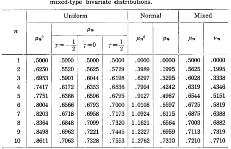
Table 1. Optimum neutral values for uniform, normal and mixed-type bivariate distributions.

Uniform Normal Mixed

"''''

",,,,0

r=--}I

r=O

_I

.5000 .5000 .5000 .6250 .5520 .5625 .6953 .5901 .6044 .7417 .6172 .6353 .7751 .6388 .6596 .8004 .6566 .6793 .8203 .6718 .6958 .8364 .6848 .7099 .8498 .6962 .7221 .8611 .7063 .7328 1 :2

r=-.

.500 .572 -) I .619 8 .653 ) .679 ) .700 ) .717 I .732 ) .744 ) .755 I ",,,,0 .0000 .3989 .6297 .7904 .9127 1.0108 1.0924 1.1621 1.2227 1.2762

"''''

_"'"

!.J" .0000 .5000 .0000 .1995 .5625 .1995 .3295 .6028 .3338 .4242 .6319 .4346 .4987 .6544 .5151 .5597 .6725 .5819 .6115 .6875 .6388 .6564 .7003 .6882 .6959 .7113 .7319 .7310 .7210 .7710

(Values of ,u",o for uniform and normal distributions were reproduced from Table 13 of [2]. Computations of values of f.In for normal distri-bution and !.J" for mixed-type distribution, were performed by exploiting Table II of Raiffa and Schlaifer [6].)

References

[1] DeGroot, M. H., Optimal Statistical Decisions, McGraw-Hill Book Co., New York, 1970, Chap. 13.

[2] Gilbert, J. P. and F. Mosteller, "Recognizing the maximum of a sequence," J. Amer. Stat. Assoc., 61 (1966), 35-73.

[3] Gumbel, E. J., "Distributions a plusieurs variables dont les marges sont donnees," C. R. Acad. Sci. Paris, 246 (1958), 2717-2720.

[4] Matsuda, T. and M. Sekiguchi, "Optimal goal levels in satisfying behavior," (in Japanese), Keiei Kagaku, 16 (1972), 88-100.

[5] Nash, J., "Non· cooperative games," Ann. 0/ Math., 54 (1951), 286-295. [6] Raiffa, H. and R. Schlaifer, Applied Statistical Decision Theory, Division of

Research, Graduate School of Bussiness Administration, Harvard University, Boston, 1961.

[7] Sakaguchi, M., "Interaction information in multivariate probability distri-butions," KODAI Math. Sem. Rep., 19 (1967), 147-155.