THE TAIL BEHAVIOR OF THE STATIONARY DISTRIBUTION OF A FLUID QUEUE WITH A GAUSSIAN-TYPE INPUT RATE PROCESS

Journal of the Operations Research Society of Japan

Vol. 40, No. 1, March 1997

THE TAIL BEHAVIOR OF THE STATIONARY DISTRIBUTION OF

A FLUID QUEUE WITH A GAUSSIAN-TYPE INPUT RATE PROCESS

Kazutomo Kobayashi Yukio Takahashi

N E C Corporation Tokyo Institute of Technology

(Received August 4, 1995; Revised October 18, 1995)

Abstract This paper deals with a fluid ueue with a Gausszan-type input rate process. The Gaussian-type

7

processes are ones defined as Rt = m

+

f _ h(t - s)dws, where m is a positive constant, w t is a standard Wiener process and h(t) is an integrable function such that h(tl2 and H ( t ) = f w h(s)ds are also integrable.

The class of Gaussian-type processes is wide enough to contain most of continuous time stochastic processes proposed so far for coded video traffic.

For the model, in this paper, the exponential decay property of the tail of the buffer content distribution is studied, and an upper bound and a lower one are given for the tail probability P ( Q w

>

X) _{of the buffer}

content distribution in the steady state. These bounds show that the tail probability decays exponentially with rate

-*,

where H(0) = :f h(t)dt and C is the output rate of the fluid queue. This result guarantees, in a sense, the plausibility of the approximation formula P ( Q w

>

X) % Bexp{-*X}

i-f(0I2/2 proposed in the previous paper [Performance Evaluation, 19951.

1.

Introduction

Asynchronous Transfer Mode (ATM) is a main technology for multiplexing and switching a variety of information such as voice, data, image and video, and the ATM technology has been adopted to High-speed Local Area Networks and to Broad-band ISDNs. Related to this movement, there have been a number of studies on performance analyses for ATM multiplexers

.

In an ATM network, information is divided into blocks of small fixed size, referred to as cells, and transmitted. For the reason, the cell arrival process at a switching node or a multiplexer has strong correlation in inter-arrival times. This strong correlation makes the stochastic structure complicated and the performance analysis difficult.

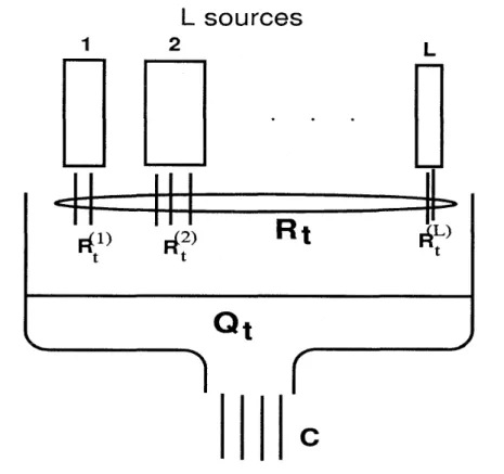
The most popular approximation which makes the stochastic structure simpler is a fluid queue model in which the detailed behavior of cells is ignored and cell streams are regarded as fluid streams (Fig. 1). In the fluid queue model, the stochastic behavior of the buffer content

Qt is represented by the differential equation

3

=

{

Rt

-

C,

if Qt

>

0 or

Rt

>

c,

dt

0, otherwise,

where

C

is a constant output rate and

Rt

is the total input rate at time

t.

Many fluid queue models studied so far assume On-Off types of traffic, in which sources have two states, On- state and Off-state, to alternate each other and each source pours fluid into the buffer at a constant rate during On-state [6, 1, 91. However, coded video traffic, which is considered to be the main traffic in ATM networks, differs largely from On-Off types of traffic.

76 K. Kobayashi & Y . Jakahashi

In some simulation studies, coded video traffic is modeled as a discrete time Gaussian process [10, 13, 7, 41. Maglaris, et al. discuss a model in which coded video traffic is rep- resented by a first-order autoregressive process [10]. With Maglaris' study as a motivation, Simonian analyzes a fluid queue model with an Ornstein-Uhlenbeck process, and obtains exact and approximate solutions [13]. Heyman, et al. discuss a model with a higher-order autoregressive process as a coded video input rate process [7], and Griinenfelder, et al. pro- pose a model with an autoregressive moving average process [4]. These processes have an advantage that the parameters of them can be easily estimated from the empirical mean and the empirical autocovariance function. However, they have been used only for simulations, and according to the authors7 knowledge, they have never been used for any theoretical analyses of fluid queue models.

There are studies on analyses of fluid queue models with Markovian-type input rate processes. Stern and Elwalid extend the On-Off source model to the one with a Markov modulated rate process (MMRP) as input rate [15]. Tanaka, et al. study the same model and obtain the transient state probabilities in an explicit form using eigenvalues and eigenvectors of a key matrix [16]. However, it is not easy to calculate the steady-state distribution from the results of these studies, except for simple fluid queue models. It is also difficult to estimate the parameters of the MMRP from actual measurement data.

In this paper, we discuss a fluid queue model with a Gaussian-type input rate process

t

defined as

Rt

= m

+

h(t - s)dws. The detailed definition is given in Section 3. The class of Gaussian-type processes is wide enough to contain most of continuous time stochastic processes proposed so far for coded video traffic such as continuous versions of autoregressive processes and autoregressive moving average processes.

For the model with a Gaussian-type input rate process, in the previous paper [g], the X] for the tail authors proposed an approximation formula

P[QW

>

X] a

B

exp[-

probability of the buffer content distribution in the steady-state, where

B

is a positive constant and H(0) =

J(?Â

h(t)dt. However, there was not given any theoretical proof for the exponential decay. The purpose of this paper is to justify the exponential decay by giving an upper bound and a lower bound which have the same exponential decay rate1. Specifically we prove that for sufficiently large X ,

where

Boy

B1

and

B2

are positive constants and

B3

is a non-negative constant.

The paper is organized as follows. In Section 2, we discuss a fluid queue model for an ATM statistical multiplexer with coded video input, and we introduce Gaussian-type input rate processes in Section 3. Section 4 is devoted to our main theorem which gives an upper bound and a lower bound for the tail probability of the buffer content distribution.

2.

Fluid Queue Model for ATM Statistical Multiplexer

We consider a fluid queue model for an ATM statistical multiplexer which accommodates multiple sources and serving with a single output line (see Fig. 1).

If

there are

L

sources and source i pours fluid into a buffer with time dependent rate

R ' ,

then the total input rate Rt is given by Rt =

~ f .

In our fluid queue model for the multiplexer, the buffer

l We note that K. Debicki and T. Rolski [3] obtain a similar upper bound for the same fluid queue model, independently

Tail Behavjor of Fluid Queue

L

sources

2

L

Figure 1: Fluid queue model for ATM statistical multiplexer

content Qt varies according to the differential equation

dQt

Rt

-

C , if Qt

>

0 or

Rt

>

C,

dt 07 otherwise,

where C is constant output rate.

Input rate

Time

ON OFF ON

Figure 2:

A

On-Off fluid model

Many fluid queue models [6,

1,

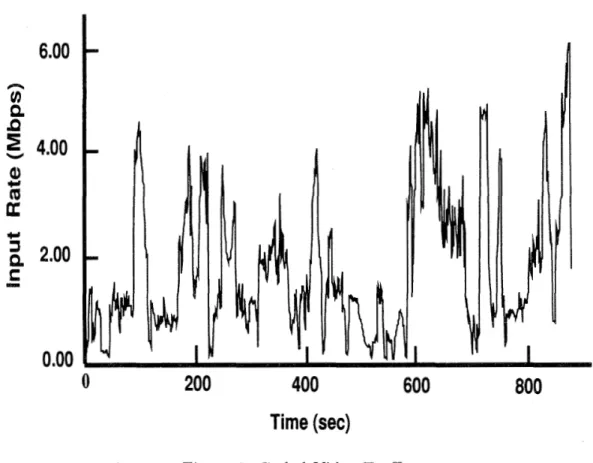
91 assume On-Off type of traffic, in which each source has two states, On-state and Off-state, to alternate each other and pours fluid into the buffer at a constant rate during On-state (see Fig. 2). Traffic from voice sources or file-transfer sources might be modeled by On-Off type processes. However, coded video traffic, which is considered to be the ma,in traffic in ATM networks, seems difficult to be modeled as an On-Off type process. Figure 3 shows an example of actual coded video traffic pattern. The vertical axis represents the input rate and the horizontal axis the time. It is much different from On-Off type of traffic.

K. Kobayashi & Y . Takahashi

Time

(sec)

Figure 3: Coded Video Traffic

In [10,

71,

video traffic is modeled as an autoregressive process

where

Xn

is the input rate at discrete time n, ak's are real constants and & ^ ' S are indepen- dently and identically distributed random variables with zero mean. The random variables cn7s are usually assumed to be normally distributed. Then, the sequence { E ~ } is considered as a discrete version of the

white

noise. The parameters a k ,

k

= 1,

- -

,

K ,

are determined

from the sample autocovariance function

A(k)

of actual measurement traffic data by using

the

Yule- Walker

equation:

The parameter uo is given by m ( l -

^{Ll

a k ) where m is the sample mean.

In [4], coded video traffic is modeled as an autoregressive moving average process,

The parameters ak's and

hi's

a,re also estimated from the sample mean and the sample autocovariance function.

Tail Behavior of Fluid Queue 79

In these processes,

X n can take negative values. So it is suggested in

[4] that the input rate is given by max(0,

X ^ ) .

However, if many video sources are multiplexed, then the standard deviation of

X n becomes relatively small compared with the mean of

Xni

and the probability that

Xn

is negative becomes negligibly small. In such cases,

X n itself can be

used as an input rate process.

These processes look complicated, but they can be rewritten in the same form

In [ll], the sequence

{h^}

for the autoregressive moving average process is given by the inverse z-transform of

Gaussian-type Input Rate Processes which will be discussed in the next section are contin- uous versions of processes of type

(2.2).

3. Gaussian-type Input R a t e Processes We discuss an input rate process

Rt

defined by

where m is a positive constant,

wt

is a standard Wiener process, and

h ( t )

is a real valued measurable function such that

h ( t )

= 0 for

t

<

0. We assume that

W here

Since

H ( t )

5

fr

\h(t)ldt

<

m , it follows that

In order to avoid trivial cases, we also assume that m is less than

C

and h ( t ) is not a function taking zero almost everywhere, so that the integrals in the inequalities (3.2) to (3.4) are strictly positive.

The process

Rt is the same as the one defined in our previous paper

[B]. Here, let us call

it

a

Gaussian-type input rate process.

Clearly, Rt is a stationary Gaussian process with

m the mean m ,

m the a~t~ocovariance function AR(r) =

j'r

h ( s

+

r )

h ( s ) d s ,

and m the variance A/

Aa(0)

=

fr

h ( t l 2 d t .

80 K. Kobayashi & Y . Takahashi

The second term in the right-hand side of (3.1) is considered as the output of a linear system with a white noise input dwt/dt and an impulse response h(t) [12]. Assumption (3.2) is the stability condition for the system, and assumption (3.3) is another essential condition in order that the integration in (3.1) exist S. These assumptions are unavoidable conditions to discuss or to construct a linear system with a white noise input. Here, we assume (3.4), too. This assumption is made to ensure for the buffer content distribution in the fluid queue model to have an exponential decay property as will be seen later. However, the assumption is not strict for practical applications since most of important stable linear systems satisfy it (see Remark 1 below).

Remark

1.

In

[8],

the authors gave some examples of h(t) satisfying (3.2), (3.3) and (3.4).

The following is a summary of those examples.

Ornstein-Uhlenbeck process

where cr is a real constant and K, is a positive constant.

Superposition of Ornstein-Uhlenbeck processes

where N is a positive integer, oi7s are real constants and K;'S are positive constants.

Continuous version of moving average process

\ h ( t ) \ < M , 0

<

t

<T,

and h(t) = 0, t

>

T,

(3.7) where

M

and

T

are positive constants.

Continuous version of autoregressive process

N

h(t) = tn2 e-Kst c o s ( ~ i t + y i ) - , t > O , i=l

(3.8) where

N

is a positive integer, ni7s are non-negative integers, 6,'s are positive constants, and oi7s, wi7s and yi7s are real constants.

Continuous version of autoregressive moving average process

where g(t) is a function of type (3.7) and

f

(t) is a function of type (3.8).

Remark

2.

In actual ATM networks, many cell streams are multiplexed, namely, many

input rate processes are superposed. Individual input rate processes may not be Gaussian- type, but the total input rate process can be expected to be close to the Gaussian-type one from the central-limit theorem. Therefore, Gaussian-type processes are thought to be widely applicable as input rate processes.

Remark 3. The mean

m

and the autocovariance function

A ^ ( T )

of an input rate process

can be estimated by the sample mean and the sample autocovariance function of actual measurement data RiAt,

i

= 1 , 2 ,

,

N,

as follows:

Jail Behavior of Fluid Queue 81

Later we will see that the quantity

H ( o ) ~ / ~

is an important factor of decay rate of the tail probability P ( Q W

>

X ) . Since

roo r o o

it is easily estimated by

N

In a fluid queue model with

L

independent input rate processes, the mean or the autoco- variance function of the total input rate process are given by the sum of those of individual input rate processes. So the decay rate can be directly estimated from the empirical means and the empirical autocovariance functions of individual sources.

4.

Bounds for the Tail Probability

P ( Q m

>

X )

In t,he previous paper [ g ] , t,he authors proposed an approximation formula for the sta- tionary tail probability as follows:

where QW is a random variable subjecting t o the steady-state distribution of the buffer content and 71 is the conditional expectation of

Rt

in the steady-state conditioned that

Rt

<

C.

In this section, we prove the following theorem which justifies, in a sense, the rate of the exponential decay in the approximation formula (4.1).

Let

At

be the

input process

defined as

Theorem

1.

Th,ere are positive constants

Bo, B1

and

B2

and a non-negative constant

B3

such that

for

sufficiently large

x,

1

C - m

C - m

exp

[-

Bo

+

B 1 f i H ( 0 ) 2 / 2 X ]

<

P(Qx

>

X )

<

( B 2

+

B 3 i ) exp[- ~ ( 0 ) ~ / ' 2 ( 4 - 3 )

where

H ( 0 )

=

fr^

h ( t ) d t . If the covariance function

Pf

between

At

-

C t and

R. is non-

negative, then the term

B3x

can

be

omitted.

We shall prove the upper bound and the lower bound separately.

4.1.

Proof of the upper bound

To get the upper bound in (4.3), we employ the following result used in Simonian and Virtamo's paper [14].

where p t ( x , y ) is the joint density function of At - C t and R o .

In [l41 ( ~ p . 1 7 3 5 (2.10)), instead of ~ ~ ( x , y)dyl the expression pt(x\y)d@(y) is used in (4.4), where p,(+) = &^'(At - C t

S

xlRO = y) and @(y) = P ( R o

5

y). Simonian and Virtamo apply (4.4) t,o the case of input rate varying as an Ornstein-Uhlenbeck pro- cess, giving h(t) = a e K t in our formulation, and obtain an upper bound in a,n explicit form.

Now let,'s consider At - C t . From (4.2) and (3.1), we have

where p =

C

- m and

TOt

=

g

dw, = wt - WO.

Since At - C t and R. are jointly Gaussian random variables, pt(x, y) is written as

where Et is a covariance matrix of the vector random variable (At - C t , Ro). The matrix

E+

is written as

where cq is the variance of At - C t

,

Qt

the covariance between At - C t and Ro7 and 7 the

variance of Ro. Then a,,

/lt

and 7 are written in terms of h(t) and H ( t ) as follows:

Lemma

1. at, Qt and 7 have the following properties:

1. at and Qt are absolutely continuous functions o f t such that 0.0 = 0 and

Q.

= 0. 2. 7 and at for t

>

0 are positive. Also

/32

<

at? for t

>

0.

3. limt^/), = H(0)'/2

>

0.

.

Let f t be a function such that at = H(Oy(t

+

f t ) , then \ { , l is bounded, and hence limt+^ at/< =

H ( O ) ~ .

5. QAt = 7 A t

+

o(At) for small A t .

6. a ~ t =

+

o ( { A ~ } ~ ) for small A t .

Proof. 1. Since H ( t ) is absolutely continuous, at and

,Bt

a,re also absolutely continuous.

Tail Behavior of Fluid Queue 83

2. Since 7 and at are the variances of

&

and

At

- C t , it is obvious that 7

>

0 and at

2

0. From the assumption that h ( t ) is not a function taking zero almost everywhere, it is easily checked that 7

>

0 and at

>

0 for

t

>

0. Since %/at'-/ is the correlation coefficient between

R.

and At - C t , the inequality

/?;

5

sty holds for t

2

0. The equality does not hold for t

>

0 since

h ( t )

is not equal to zero almost everywhere.

3. Since limt+cc H ( t

+

S ) = 0 , the limit of (4.7) is given by

lim

t-cc = i W H ( s ) h ( s ) d s

4. We evaluate H ( 0 ) 2 & = at - w t . From (4.6), we have

From (3.2), (3.3), (3.4) and (3.6), the right-hand side of the above inequality is finite. 5. By differentiating (4.7), we have

It is easily checked from (3.3) that A R ( t ) is continuous at

t

= 0. Note that = 0 and

/?A

= A R ( 0 ) = 7 . Using Taylor's formula, we have

6. By differentiating (4.6), we have

84 K. Kobayashi & Y . 7akahashi

Now we return to (4.5). Rearranging the term in the brackets, we have

Substituting pt(x7 y ) in (4.4) with (4.9), we have

Then the right-hand side of (4.10) is represented as

For 0

<

t

<

m, the following inequality holds:

Lemma

2. Let xo be an arbitrarily fixed positive number. Then, there exist a positive

constant

D1

and a non-negative constant

D2

such that for X

>

x0 and

t

>

0

If

A

2

0 for

all

t

>

0 , then we may put

D2

= 0 . Proof.

We

write .q as

Z t =

f

( t )

+

g ( t ) ( x - xo),

Jail Behavior o f Fluid Queue 85

From Lemma 1,

y

- g/at is positive for t

>

0 and bounded from above by

y.

We note that

B2 0

limt+o(y - 2 ) = 0, limt+o(l - Ã ‘ t = 0, and limt+o ,&/at = + m . Hence we have

at at

On the other hand, it is easily checked that fi

lim

f

(t) =

-

lim g(t) = 0,

t+O0 2,/7' t+w

since limt^ = 0, limt+OO ^/at = 0, limt+OO /?t = H(0)2/2 and limt+OO a t / t =

Functions

f

(t) and g(t) are continuous and they are bounded from above. If we set D 2 =

supt>o g(t) and Dl =

f

( t ) - D2x0, then

Dl

and D 2 are finite and the inequality (4.12)

holds.

If

2

0 for all t

>

0, then g(t)

<:

0 and hence

D2

= 0. From the inequality (4.11) and Lemma 2, we have

To evaluat'e the integrand in m ( t

+

St). From Lemma 1,

1^1.

Lemma

3. Let 6 be an arbitrary

O0 1

+

D ~ X 27~ o ) P /

ex^[-

( X

+

i i t y

]

dt.

2%

the right-hand side of (4.13)) we shall replace 0.1 with is a bounded function and we let

f

is an upper bound of positive number. Then, for X

>

pf

+

612 and t

>

0,

where

D3

= H(O)/^/-.

Proof. Let F ( t ) be the ratio of the right and the left sides of (4.14), namely,

( X

+

i i q 2 + (X

+

fit -

e x p [ 2 ~ ( 0 ) 2 ( t + y 2 H ( 0 l 2 ( t + f )

1.

Since t

+

f ,

<

t

+

f ,

it is less than

The numerator in the brackets is divided as 6(x

+

fit - 612) = 6(x - pf - 612)

+

fiS(t

+

f ) ,

and we have

where

0

= (t

+

f ) / ( t

+

&).

The function f l e x p [ - m ] is concave on [O, m ) and has maximum value

Ds

=

86

Lemma

4.

K. Kobayashi & Y . Takahashi

27rH 0

where D4

= _exp

[c2

_(:

+

_{f ) ]}

_.

Proof.

Let

<

=

t

+

{,

c

=

JTi/

H ( 0 )

and

i

= ( X -

A

-

p ( ; ) / p .

Then the left-hand side of

(4.15)

is written as

By extending the integral region to (0, oo) and by applying the well-known formula

we have an upper bound

^TT

-

e x p [ - 2 c 2 i ]

=

D4

exp

[-

P

c

~ ( 0 ) ~ / 2 ~ ^

where

Applying Lemmas

3

and

4

to

(4.13),

we have for X

>

pf

+

812,

where

B 2

=

D4LIi

J-y/2ir

and

By

=

~ ~ ~ ~ 4 5 .

If

,Of

>

0

for all

t

>

0, then we may set

D2

=

0

a n d hence

B y

=

0.

Remark 4.

Recall that

,Bo

= 0 and

,B,

=

A ^ ( ^ ) .

Then,

,Bt

is rewritten as

In case of an Ornstein-Uhlenbeck process,

A^(<)

is always positive and hence

,Bt

is always positive. Hence

B3

in the upper bound may be set to zero. When actual measurement data

i

=

I , 2,

- ,

TV,

are given, we can also judge whether

,&

is always positive or not, by accumulating the sample autocovariance of

RiAt7

i

=

I , 2,

-

.

-

,

N .

4.2.

Proof of the lower bound

Lemma

5.

The tail distribution of the buffer content

Qoo in the steady-state satisfies

Tail Behavior of Fluid Queue 87

Proof.

According to [2, 51, the solution of the differential equation (2.1) with Q. = 0 is

written as Qt = At - C t - inf {As - CS} 0<s<t Let = t - S, then Thus

Q i

= sup {A,- - C?}. 0<t<t

P ( Q m

>

X ) = lim

P(

sup {A, -

cT}

>

X ) = P(sup{At - Ct}

>

X).

t-+m _{o a t t>0}

Since { ~ u p , > ~ { A ~ - C t }

>

X} 3 {At - C t

>

0, t E [0, m)}, we have for arbitrary t

>

0

Hence we have the inequality (4.16). D

Since At - C t is a Gaussian process, P ( A t - C t

>

X ) is given by

where

X

+

p t 1 U

~t =

-

and G(y) =

-/

exp[--]due

IF

' 1 v Y

2

Note that

it

is a function such that at = H(0)2(t

+

f,). From Lemma 1, there exists

f

such that

l&l

< { < m .

F o r t

>

{let

then we have the following lemma.

Lemma

6 .

P(QW

>

X)

>

G(min ijt). t>S,

Proof.

From

\[,\

<

f <

m, we have

X

+

p t X

+

p t

=

JB{oyo

<

JH(oy(t

=

for t

> f .

Since $(y) is a decreasing function of y, 6 ( y t ) is greater than

$(gt)

for all t

> f .

Then, from (4.16) and (4.17), we have

88 K. Kobayashi & Y . Takahashi

Using (4.19) and the inequality

we have

1

P(Qm

>

X )

>

^'-

lix

+

PT]

H(0)2/2

.

G(*-

+

l )

Since

\

/

a

x

<

s

<

+

&

for a

>

0,

b

>

0 and x

>

0, we obtain the desired lower bound

References

D. Anick, D. Mitra and M. M. Sondhi, Stochastic Theory of a Data-Handling System with Multiple Sources,

The Bell System Technical Journal

61(8) (1982) 1871-1894. V.

E.

Benes,

General Stochastic Processes in the Theory of Queues

(Addison-Wesley, Reading, MA, 1963).

K. Debicki and T . Rolski, A Gaussian Fluid Model,

Queueing Systems

2 0 (1995) 433- 452.

R. Griinenfelder,

J.

P. Cosmas, S. Manthorpe and A. Odinma-Pkafor, Characterization of Video Codecs as Autoregressive Moving Average Processes and Related Queueing System Performance,

IEEE

J. Set. Areas in Commun.

9(3) (1991) 284-293.

J.

M. Harrison,

Brownian Motion and Stochastic Flow Systems

(Wiley, New York, 1985).

0 . Hashida and

M.

Fujiki, Queueing Models for Buffer Memory in Store-and-Forward System,

Proc.

ITC-7,

(1973) 323/1-323/7.

D. P. Heyman, A. Tabatabai and T . V. Lakshman, Statistical Analysis and Simulation Study of Video Teleconference Traffic in ATM Networks,

IEEE

Trans. on Circuits and

Systems for Video Tech.

2(1) (1992) 49-59.

K. Kobayashi and Y. Takahashi, Steady-State Analysis of ATM Multiplexer with Variable Input Rate through Diffusion Approximation,

Performance Evaluation

23(2) (1995) (to appear).

L.

Kosten, Stochastic Theory of Data Handling Systems with Groups of Multiple Sources,

Performance of Computer-Communication Systems

(North-Holland, 1984) 321-331.

B.

Maglaris, D. Anastassiou, P. Sen,

G.

Karlsson and J . D. Robbins, Performance Models of Statistical Multiplexing in Packet Video Communications,

IEEE

Trans. on

Commun.

36(7) (1988) 834-843.

A. V. Oppenheim and R. W. Schafer,

Digital Signal Processing

(Prentice-Hall, New Jersey, 1975).

A. Papoulis,

Probability, Random Variables, and Stochastic Processes

(McGraw-Hill, New York, 1965).

Tail Behavior of Fluid Queue 89

[l31 A. Simonian, Stationary Analysis of a Fluid Queue with Input Rate Varying as an Ornstein-Uhlenbeck Process,

SIAM

J. Appl. Math.

51(3) (1991) 828-842.

[l41 A. Simonian and

J.

Virtamo, Transient and Stationary Distributions for Fluid Queues and Input Processes with a Density,

S I A M J. Appl. Math.

51(6) (1991) 1732-1739. [l51

T.

E. Stern and A.

I.

Elwalid, Analysis of Separable Markov-Modulated Rate Models

for Information-Handling Systems",

Adv. Appl. Prob.

2 3 (1991) 105- 139.

[l61 T. Tanaka, 0 . Hashida and

Y.

Takahashi, Transient Analysis of Fluid Model for ATM Statistical Multiplexer,

Performance Evaluation

23(2) (1995) 145- 162.

Kazutomo KOBAYASHI

C&C Research Laboratories, NEC Corporation 4- 1- 1 Miyazaki, Miyamae-ku, Kawasaki 21 6, Japan e-mail: [email protected]

Yukio TAKAHASHI

Mathematical and Computing Sciences Tokyo Institute of Technology

2-12-1 Oh-Okayama, Meguro-ku, Tokyo 152, Japan e-mail: yukio@is. titech.ac.j p