線形分離オートマトンの高速な状態数最小化アルゴリズム

全文

(1)Vol.2010-MPS-79 No.3 2010/7/12. 情報処理学会研究報告 IPSJ SIG Technical Report. 1. Introduction. 線形分離オートマトンの高速な状態数最小化アルゴリズム沼井裕二†1. 小林. The theory of computational models that can deal with sequences of real valued vectors is an important research topic if we consider problem domains including weather forecasting5) , motion recognition3),4) , and time-sequential image analysis9) . We proposed a computational model, called a Linear Separation Automaton (LSA for. 聡†1. short). The LSA is an extended model of a finite automaton. It accepts a sequence of real vectors, and has a weight and a threshold sequence at every state, which determine. 本論文では，著者らが過去に提案した線形分離オートマトン（LSA）の状態数最小化アルゴリズムを高速化する．LSA は有限オートマトンを拡張したモデルで，実ベクトル系列を受理する能力を持ち，各状態には重み関数と閾値系列が付随する．この二つによって，各時点でのある状態からの遷移先状態が決定する．過去の著者らの論文では，与えられた LSA M の状態数を最小化する理論を確立し， O(n2 ) 時間の状態数最小化アルゴリズムを提出した．n は M の状態数である．本論文では， O(n log n) 時間にまで高速化した状態数最小化アルゴリズムを与える．. the transition from the current state to the next at each step. If we consider the learning problem of automata, it is essentially important to establish the theory of minimizing the number of states of a given automaton. It is often the case that learning algorithms try to find a minimum state automaton consistent with a given set of examples. In our previous works, we established a theory of minimizing the number of states of a given LSA7) , and proposed an O(n2 ) time state minimization algorithm6) . This paper gives an O(n log n) time efficient state minimization algorithm of a given LSA.. Efficient State Minimization Algorithm of Linear Separation Automata Yuji Numai†1 and Satoshi Kobayashi. 2. Preliminaries In this section, we introduce some basic definitions and notation, and introduce a. †1. linear separation automaton. 2.1 Basic Definitions and Notation. In this paper, we present a faster state minimization algorithm of a linear separation automaton (LSA for short) than the algorithm we recently proposed. An LSA is an extended model of a finite automaton. It accepts a sequence of real vectors, and has a weight and a threshold sequence at every state, which determine the transition from the current state to the next at each step. We established a theory of minimizing the number of states of a given LSA M , and proposed an O(n2 ) time state minimization algorithm of M , where n is the number of states of M . This paper gives an O(n log n) time efficient state minimization algorithm of M .. By R, we denote the set of real numbers. For a positive integer d, by Rd we denote d-dimensional vector space over R. For x, y ∈ Rd , x ⊗ y denotes the inner product of x and y. We define (Rd )∗ as the set of all finite sequences of elements in Rd . For a sequence α = ⟨x1 , . . . , xn ⟩ ∈ (Rd )∗ , we denote the length of α by |α|, i.e., |α| = n. An element in (Rd )∗ of length 0 is called an empty sequence, and is denoted by λ. For sequences α, β ∈ (Rd )∗ , we denote the concatenation of sequences α and β by αβ. For α = ⟨x1 , . . . , xn ⟩ ∈ (R1 )∗ , α is said to be increasing if the inequality xi < xi+1 holds for every i. Let S be a set. A partition π = {S1 , . . . , Sk } of S is the set of mutually disjoint. †1 電気通信大学大学院電気通信学研究科情報工学専攻 Department of Computer Science, Graduate School of Electro-Communications, The University of Electro-Communications. non-empty subsets Si of S for 1 ≤ i ≤ k such that ∪i=1,...,k Si = S. A partition π = {S1 , . . . , Sk } of Rd is said to be linearly separable iff there exist w ∈ Rd and an. 1. c 2010 Information Processing Society of Japan ⃝.

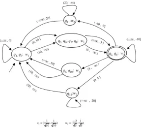
(2) Vol.2010-MPS-79 No.3 2010/7/12. 情報処理学会研究報告 IPSJ SIG Technical Report. increasing h = ⟨h1 , . . . , hk−1 ⟩ ∈ (R1 )∗ such that, for any x ∈ Rd , hi−1 < w ⊗ x ≤ hi. δ(q, x) = s(q)1 . Finally, assume that |s(q)| ≥ 2. The value δ(q, x) is defined as follows:   s(q) if w(q) ⊗ x ≤ h(q)1 1 . ⇔ x ∈ Si (i = 1, . . . , k).     s(q)2   . holds, where h0 = −∞ and hk = ∞.. .. δ(q, x) = .     s(q)iq. Consider equivalence relations ≡, ≡1 , and ≡2 over (Rd )∗ . The number of the equivalence classes of ≡ is called the index of ≡. An equivalence relation ≡1 is finer than an.   . equivalence relation ≡2 (or ≡2 is coarser than ≡1 ) iff x ≡1 y implies x ≡2 y for any x. if. h(q)1 < w(q) ⊗ x ≤ h(q)2 .. .. if h(q)iq −1 < w(q) ⊗ x ≤ h(q)iq. s(q)iq +1 if h(q)iq < w(q) ⊗ x . Consider a state transition diagram as in Fig. 1. Suppose that δ(q, x) = p holds if. and y. An equivalence relation ≡ is right invariant iff α ≡ β implies αγ ≡ βγ for any. h(q)i < w(q) ⊗ x ≤ h(q)i+1 . In the diagram, the transition from q to p is associated. α, β and γ.. with the interval (h(q)i , h(q)i+1 ].. d. Consider partitions π1 and π2 of R . A partition π1 is finer than a partition π2 (or π2 is coarser than π1 ) iff for any block B1 ∈ π1 , there exists a block B2 ∈ π2 such that. For α = ⟨x1 , . . . , xl ⟩ ∈ (Rd )∗ , we write δ(p, α) = q if there exists a sequence. B1 ⊆ B2 . We say that π1 is a refinement of π2 iff π1 is finer than π2 . 2.2 Linear Separation Automata. p1 (= p), p2 , . . . , pl+1 (= q) of states such that δ(pi , xi ) = pi+1 holds for any i. We. A linear separation automaton (LSA) M is formally defined as an 8-tuple. define the set of sequences accepted by an LSA M , denoted by L(M ), as L(M ) = {α ∈ (Rd )∗ | δ(q0 , α) ∈ F }. A subset L of (Rd )∗ is said to be regular if there exists an LSA. M = (d, Q, q0 , F, w, h, s, δ) ,. M such that L = L(M ). We define the size of M as the cardinality |Q| of Q.. where d is a positive integer specifying the dimension of input vectors to M ; Q is a finite. A state q ∈ Q is said to be reachable if there exists α ∈ (Rd )∗ such that δ(q0 , α) = q.. set of states; q0 is an initial state (q0 ∈ Q); F is a finite set of final states (F ⊆ Q); w. A state q ∈ Q is said to be unreachable if q is not reachable.. is a weight function from Q to Rd such that w(q) is a unit vector for any q ∈ Q; h is a threshold function from Q to (R1 )∗ such that h(q) is increasing for every q ∈ Q, and. Example 1. Consider an LSA M1 in Fig. 1. Let α = ⟨x1 , x2 , x3 ⟩ be an input sequence √ √ √ √ √ √ of vectors in R2 with x1 = (3 10, 2 10), x2 = (− 5, 2 5), and x3 = (−3 10, −2 10).. is denoted by h(q) = ⟨h(q)1 , . . . , h(q)|h(q)| ⟩; and s is a sub-transition function from Q ∗. to Q , and is denoted by s(q) = ⟨s(q)1 , . . . , s(q)|s(q)| ⟩. If |s(q)| ≥ 1, then the equality. It holds that δ(q1 , x1 ) = q6 , δ(q6 , x2 ) = q4 , and δ(q4 , x3 ) = q4 ∈ F . Hence, the sequence. |h(q)| = |s(q)| − 1 holds for every q ∈ Q.. α is accepted by M1 . In order to improve the readability, we write iq = |h(q)| for any q ∈ Q.. 3. Basic State Minimization Algorithm of LSA. δ is a state transition function from Q × Rd to Q; and is defined in the following way by using w, h, and s. Consider any state q ∈ Q and vector x ∈ Rd . The definition. In this section, we give some theoretical results for LSAs, showed in 7), and review a. of δ is separated into three components. First, in the case of |s(q)| = 0, the value. basic algorithm to minimize the number of states of a given LSA, presented in 6).. δ(q, x) is undefined. Secondly, suppose that |s(q)| = 1. The value δ(q, x) is defined as. 3.1 Theoretical Results For any subset S of (Rd )∗ , we define an equivalence relation ≈S over (Rd )∗ as follows: α ≈S β. def. ⇔. ∀γ ∈ (Rd )∗ (αγ ∈ S iff βγ ∈ S) .. Let M = (d, Q, q0 , F, w, h, s, δ) be an LSA accepting S with no unreachable states.. 2. c 2010 Information Processing Society of Japan ⃝.

(3) Vol.2010-MPS-79 No.3 2010/7/12. 情報処理学会研究報告 IPSJ SIG Technical Report (20,. w(q1 ) = w(q2 ). A state q1 is preceding to a state q2 with respect to a state q, denoted by. ). q1 ≺q q2 , if there exists an integer i such that s(q)i = q1 and s(q)i+1 = q2 . For q ∈ Q,. (-10 , 0 ]. q11:w2. we define. , 0]. For a subset X of Q, we define ∆(X) = { p | q ∈ X, p ∈ ∆(q) } .. (10 ,. (5 ,. For a partition π of Q and q1 , q2 ∈ Q, we write q1 ∼(π) q2 if there exists B ∈ π such. , 20] 0, ). ) ,2 0]. ). (0,. q3:w1. 5]. ( (0,. w1 = (. For a subset X of Q and ω ∈ W (Q), we define Xω = { q ∈ X | w(q) = ω } .. , 0]. q12:w2. 5]. 3 1 , ) 10 10. W (X) = { w(q) | q ∈ X } .. ). q8:w2 , -10]. that q1 , q2 ∈ B. For a subset X of Q, we define. ,. (20,. (. (5. , (20. q4:w1. (1. q7:w1. (. 0] ,1. (0,5]. ( (. (5 ,. ). ,2 0]. 0] (-10 ,. ). ,. q9:w2. (. (. ∆(q) = { p | p ∈ s(q) } .. q2:w1 ). ( 20. q6:w2 ). q10:w1. , -10]. ]. ) ). , (20. , 10]. ,5. ). ] , 20. (0 (1 0 ,. q1:w1. (. (. q5:w1. ] , 10. (5 ,. (. (. w2 = (. −2 1 , ) 5 5. (. For any ω ∈ W (Q), we also define H(ω) = { h(q)i | q ∈ Qω , 1 ≤ i ≤ iq , s(q)i ̸= s(q)i+1 } ∪ {∞} .. , 20]. For ω ∈ W (Q) and v ∈ H(ω) , we define the function δω,v from Qω to Q as follows: δω,v (q) = δ(q, x) for some x ∈ Rd with ω ⊗ x = v .. Fig. 1 LSA M1 .. We define the set of functions ∆ as follows: For any p, q ∈ Q, there exists α, β ∈ (Rd )∗ such that δ(q0 , α) = p and δ(q0 , β) = q. We. ∆ = { δω,v | ω ∈ W (Q), v ∈ H(ω) } .. define the equivalence relation ∼ over Q as follows:. In the sequel, for simple description of the algorithm, we often use graph representa-. def. p ∼ q ⇔ α ≈S β .. tion of mappings f ∈ ∆ and ∆ : Q → 2Q , i.e., f is represented as a graph containing. The states p and q are said to be indistinguishable iff p ∼ q. The states p and q are. edges between q1 and q2 such that q2 = f (q1 ), written q1 f q2 ; and ∆ is represented as a. said to be distinguishable iff p ̸∼ q.. graph containing edges between q1 and q2 such that q2 ∈ ∆(q1 ), written q1 ∆q2 .. For any p ∈ Q, by r(p) we denote a representative element of [p]∼ . We define an Theorem 2 (Characterization of Partition Q/ ∼). Let M = (d, Q, q0 , F, w, h, s, δ) be. LSA M/ ∼= (d, Q′ , q0′ , F ′ , w′ , h′ , s′ , δ ′ ) ,. an LSA. The partition Q/ ∼ is a coarsest refinement π of π0 = {F, Q − F } which satisfies the following conditions:. where Q′ = Q/ ∼ , q0′ = [q0 ]∼ , F ′ = {[q]∼ | q ∈ F } ,. (C1) ∀B ∈ π ∀f ∈ ∆ ∃B ′ ∈ π such that f (B) ⊆ B ′ ,. δ ′ ([q]∼ , x) = [δ(r(q), x)]∼ , w′ ([q]∼ ) = w(r(q)) , h′ ([q]∼ ) = h(r(q)) .. (C2) ∀B ∈ π ( |W (B)| > 1 ⇒ ∃B ′ ∈ π such that ∆(B) ⊆ B ′ ) .. Theorem 1 (Characterization of Minimum State LSA). Let M be an LSA. The LSA Now, let us describe the basic state minimization algorithm of a given LSA. It uses. M/ ∼ is a minimum state LSA for M such that L(M/ ∼) = L(M ).. two primitive refinement operations split1 and split2 ; the former is for the condition. 3.2 Basic State Minimization Algorithm. (C1), and the latter is for (C2).. Let M = (d, Q, q0 , F, w, h, s, δ) be an LSA. For a state q1 , q2 ∈ Q, we write q1 ∼w q2 if. 3. c 2010 Information Processing Society of Japan ⃝.

(4) Vol.2010-MPS-79 No.3 2010/7/12. 情報処理学会研究報告 IPSJ SIG Technical Report. (20,. ). Algorithm 1 Basic State Minimization Algorithm for LSA , 20]. (. (. , 0]. (0. ] , 10. ( -10. (. q5, q6, q7, q8: w1. (10,. q1, q3: w1. q11:w2. (. Input: An LSA M = (d, Q, q0 , F, w, h, s, δ) , 0]. ,5]. (5 ,. ). , 10 ]. , -10]. q2, q4: w1. ). ). let π = {F, Q − F };. 2:. loop. 4: (0,. 5]. 5:. (20 , ). 1:. 3:. ) (5 ,. q9, q10: w1. (10 ,. Output: π (. 6:. q12:w2 (. , 20]. 7: 8:. w1 = (. 3 1 , ) 10 10. w2 = (. −2 1 , ) 5 5. 9: 10:. Fig. 2 Minimum state LSA of M1 .. For a set S ⊆ Q, f ∈ ∆, and a partition π of Q, the operation split1 (S, f, π) is defined. if ∃ B ∈ π such that split2 (B, π) ̸= π then replace π with split2 (B, π); else if ∃ B ∈ π, ∃ f ∈ ∆ such that split1 (B, f, π) ̸= π then replace π with split1 (B, f, π); else output π and halt; end if end loop. Example 2. The output of Algorithm 1 for the input LSA M1 in Fig. 1 is in Fig. 2.. as follows:. 3.3 Correctness of Algorithm 1 We give some basic properties of the split operations:. find all blocks B ∈ π such that f (B) ∩ S ̸= ∅ and f (B) ̸⊆ S. Define B1 = B ∩ f −1 (S) and B2 = B − B1 . Then, split B ∈ π into the blocks B1 and B2 , which results in the. Lemma 1. A partition π satisfies (C1) if and only if split1 (B, f, π) = π for every. refinement of π.. block B ∈ π and f ∈ ∆. A partition π satisfies (C2) if and only if split2 (B, π) = π for every block B ∈ π.. For a set S ⊆ Q and a partition π of Q, the operation split2 (S, π) is defined as follows:. Lemma 2. If π2 is a refinement of π1 and split1 (S, f, π1 ) = π1 holds, then split1 (S, f, π2 ) = π2 holds. If π2 is a refinement of π1 and split2 (S, π1 ) = π1 holds,. find all blocks B ∈ π such that ∆(B) ∩ S ̸= ∅, ∆(B) ̸⊆ S and |W (B)| > 1, and split B. then split2 (S, π2 ) = π2 holds.. into some smaller blocks defined in the following way; Define B ′ = { q ∈ B | ∆(q) ∩ S ̸=. Lemma 3. The equalities split1 (S1 , f, π) = π and split1 (S2 , f, π) = π imply. ∅ and ∆(q) ̸⊆ S }, B1 = {q ∈ B − B ′ | ∆(q) ⊆ S}, and B2 = (B − B ′ ) − B1 . For each. split1 (S1 ∪ S2 , f, π) = π. The equalities split2 (S1 , π) = π and split2 (S2 , π) = π im-. ω ∈ W (B ′ ), consider Bω′ . Then, split B ∈ π into B1 , B2 and Bω′ ’s for all ω ∈ W (B ′ ),. ply split2 (S1 ∪ S2 , π) = π.. which results in the refinement of π.. Lemma 4. If π1 is a refinement of π2 and split2 (S, π2 ) = π2 holds, then split1 (S, f, π1 ) is a refinement of split1 (S, f, π2 ).. Algorithm 1 is below.. Lemma 5. Let π1 be a partition satisfying (C1) and S be a union of some blocks in. 4. c 2010 Information Processing Society of Japan ⃝.

(5) Vol.2010-MPS-79 No.3 2010/7/12. 情報処理学会研究報告 IPSJ SIG Technical Report. π1 . If π1 is a refinement of π2 , then split2 (S, π1 ) is a refinement of split2 (S, π2 ).. 4. Efficient State Minimization Algorithm. Lemma 6. Algorithm 1 maintains the invariant that any coarsest refinement of the initial partition {F, Q − F } satisfying (C1) and (C2) is also a refinement of the current. In this section, we will show a faster algorithm than Algorithm 1, called Algorithm. partition π.. 2, which works in time O(m log n) = O(Kn log n). This is based on the “process the smaller half” idea used by Hopcroft1),2) and Paige8) .. Finally, we have the following theorem.. In Algorithm 2, we keep two partitions π and π ′ such that π is a refinement of π ′. Theorem 3 (Correctness of Algorithm 1). Let M = (d, Q, q0 , F, w, h, s, δ) be an LSA,. and split1 (B, f, π) = π and split2 (B, π) = π hold for every block B ∈ π ′ and f ∈ ∆. A. and n = |Q|. Algorithm 1 for the input M is correct and terminates after at most n − 1. block B ∈ π ′ is said to be compound if it contains more than one blocks of π.. refinement steps, having computed the coarsest refinement of {F, Q−F } satisfying (C1) and (C2).. Algorithm 2 Efficient State Minimization Algorithm for LSA. Proof. Since the number of blocks of a partition of Q is less than or equal to n, and. Input: An LSA M = (d, Q, q0 , F, w, h, s, δ). since the number of blocks increases at each refinement step, the algorithm terminates. Output: π. at most n − 1 refinement steps. Lemma 1 implies that the final partition πf satisfies. 1:. let π = {F, Q − F };. (C1) and (C2). Moreover, Lemma 6 implies that πf should be the coarsest refinement. 2:. let π ′ = {Q};. of {F, Q − F } satisfying (C1) and (C2).. 3:. while π ̸= π ′ do. Let us discuss the time complexity of Algorithm 1. We define K = max{ |H(ω)| | ω ∈ W (Q) } and. 4:. select a compound block B ∈ π ′ ;. 5:. let B1 , B2 be the first two blocks of π contained in B, and let B1 be the smaller;. 6:. let π ′ := (π ′ − {B}) ∪ {B1 , B − B1 };. 7:. if split2 (B1 , π) ̸= π then replace π with split2 (B1 , π);. 8:. k = max{ |∆(q)| | q ∈ Q } .. end if. The following theorem holds.. 9:. Theorem 4 (Time Complexity of Algorithm 1). Let M = (d, Q, q0 , F, w, h, s, δ) be. 10:. an LSA, and n = |Q|.. 11:. The time complexity of Algorithm 1 for the input M is. 12:. 2. O((K + k) n ). Proof. Let m = (K + k)n, i.e., m is the upper bound of the total number of edges. for all f ∈ ∆ such that split1 (B1 , f, π) ̸= π do replace π with split1 (B1 , f, π); end for. 13:. end while. 14:. output π;. contained in the graphs f ∈ ∆ and in the graph ∆. It is straightforward to see that finding a block B satisfying the if-conditions (at lines 3 and 5) and refining π afterwards. Note that at lines 8 and 11 of Algorithm 2, π might be refined by split operations, and that at line 6 π ′ might be refined by decomposing a compound block. Therefore,. can be done in time O(m). Moreover, the upper bound of the number of refining π is n − 1.. at every while loop, π is a refinement of π ′ , and there exists a compound block in π ′. Hence the time complexity of Algorithm 1 is O(mn) = O((K + k) n2 ).. unless π = π ′ .. 5. c 2010 Information Processing Society of Japan ⃝.

(6) Vol.2010-MPS-79 No.3 2010/7/12. 情報処理学会研究報告 IPSJ SIG Technical Report. The correctness of Algorithm 2 can be proved almost in a similar manner as in the. B1. case of Algorithm 1. An important difference is that in Algorithm 2, we apply only. size1 size2. split1 and split2 operations based only on B1 , and do not apply those operations based on B − B1 . However, we can show that the latter operations are not necessary for the. w1. size. q1. q2. q3. construction of the coarsest refinement.. w2. size. q4. q5. q6. w3. size. q7. q8. w1. size. q9. q10. w3. size. q11. w1. size. q12. B2. Lemma 7. Let S be any subset of Q, π be a partition of Q, B be a block in π with. size1 size2. B ⊆ S, and f be a function in ∆. (1) If split1 (S, f, π) = π holds, split1 (B, f, π) = split1 (S − B, f, split1 (B, f, π)) holds.. B3. (2) If split2 (S, π) = π holds, split2 (B, π) = split2 (S − B, split2 (B, π)) holds.. size1 size2. ′. Proof. We will show the proof of (1). Let π = split1 (B, f, π). Let D be any block in. S1. π ′ . We will prove that either f (D) ⊆ S − B or f (D) ∩ (S − B) = ∅ holds.. CL. size. Note that π ′ = split1 (B, f, π ′ ) holds. Therefore, for any D ∈ π ′ , f (D) ⊆ B or f (D) ∩ B = ∅ holds.. S2. In the case of f (D) ⊆ B, we have f (D) ∩ (S − B) = ∅. Let us consider the case. size. Fig. 3 Data Structure.. of f (D) ∩ B = ∅. By split1 (S, f, π) = π and Lemma 2, split1 (S, f, π ′ ) = π ′ holds. Therefore, f (D) ⊆ S or f (D) ∩ S = ∅ holds. In the case of f (D) ∩ S = ∅, we have. at each step, the current partition π is a refinement of the coarsest one. Then, we can. f (D) ∩ (S − B) = ∅. In the case of f (D) ⊆ S, by combining with f (D) ∩ B = ∅, we. show that Algorithm 2 outputs the coarsest refinement after at most n − 1 refinement. obtain f (D) ⊆ S − B.. steps.. In conclusion, for any D ∈ π ′ , we have either f (D) ⊆ S − B or f (D) ∩ (S − B) = ∅. Therefore, split1 (B, f, π) = split1 (S − B, f, π ′ ) holds. The proof of (2) can be obtained in a similar way.. In the case of Algorithm 2, each state always moves to a block which is smaller than half of the current one, therefore, each state can move from a block to a block at most O(log n) times. Furthermore, using the data structure in Fig. 3, we can implement. Theorem 5 (Correctness of Algorithm 2). Let M = (d, Q, q0 , F, w, h, s, δ) be an LSA,. the inner blocks of the while loop in O(m + |B1 |) time. If we notice that each edge is. and n = |Q|. Algorithm 2 for the input M is correct and terminates after at most n − 1. processed at most O(log n) times, the total time complexity is bounded by O(m log n). refinement steps, having computed the coarsest refinement of {F, Q−F } satisfying (C1). time.. and (C2). Proof. We can show by induction and with Lemma 7 that, at each iteration of the while. We will describe several data structures necessary for the implementation of Algo-. loop, split1 (B, f, π) = π and split2 (B, π) = π hold for any B ∈ π ′ and f ∈ ∆, and that. rithm 2. We will describe each element x by a record, which we shall not distinguish. 6. c 2010 Information Processing Society of Japan ⃝.

(7) Vol.2010-MPS-79 No.3 2010/7/12. 情報処理学会研究報告 IPSJ SIG Technical Report. later resetting. If S ′′ ∈ π ′ containing D becomes compound, then add S ′′ to CL.. from the element itself. We represent each pair x, y such that x f y or x ∆ y by a record, which is called an edge. Each edge x f y and x ∆ y points to element x. Each element. (4). and f (D) ̸⊆ B1 , split D into D1 = D ∩ f −1 (B1 ) and D2 = D − D1 . Do this by. y points to a list of the edges x f y and a list of edges x ∆ y. This allows the scanning of the set f. −1. ({y}) or ∆. −1. For all f ∈ ∆, do the following procedure. For each D ∈ π such that f (D)∩B1 ̸= ∅ scanning edges x f y such that y ∈ B1 . To process an edge x f y with y ∈ B1 ,. ({y}) in time proportional to its size. ′. Concerning partitions π and π , we need data structures described in Fig. 3. A block. determine D ∈ π and ω ∈ W (D) such that Dω contains x, create a temporary. B of π is represented as a record containing its sizes |B| and |W (B)| (indicated by size1. block Dω′ for Dω and move x from Dω to Dω′ . After scanning, a new block con-. and size2, respectively, in Fig. 3), and a doubly linked list containing pointers to records. taining only Dω′ is added to π if Dω is not empty, Dω is just replaced by Dω′. of Bω ’s for all ω ∈ W (B). Each Bω is represented as a record containing its weight ω,. otherwise (i.e., no change on Dω ), where size information is also updated appro-. its size |Bω |, a pointer to the record B and a doubly linked list of states contained in. priately. Temporary blocks Dω′ are linked together and have pointers to their. it. Each member (state) in the list also points to the record Bω . For a block S of π ′ ,. original blocks Dω for later process on them. If S ′′ ∈ π ′ containing D becomes. ′. compound, then add S ′′ to CL.. we define Blk(S) = {B ∈ π | B ⊆ S}. A block S of π has a record containing its size |Blk(S)| and a doubly linked list of pointers to records of blocks in Blk(S), where the. The correctness of the implementation follows in a straightforward way from our. records of blocks in Blk(S) also points to the corresponding elements of this list. Each. discussion above.. element (pointer) of the list also points to the record S. We also maintain a doubly linked list CL of pointers of compound blocks of π ′ .. Theorem 6 (Time Complexity of Algorithm 2). Let M = (d, Q, q0 , F, w, h, s, δ) be an LSA, and n = |Q|. The time complexity of Algorithm 2 for the input M is O(Kn log n).. We can implement Algorithm 2 in the following way. (1). Remove a compound block S from CL. If there exists no compound blocks, out-. Proof. The preprocess for data structure at the initialization stage requires only. put π and halt. Otherwise, examine the first two blocks in S and let B1 be the. O(m + n) time. The time spent in a refinement step is O(1) per edge scanned plus O(1). smaller. (2). per vertex of B1 , which results in the total time complexity O(m log n) = O(Kn log n),. Remove B1 from S and create a new block S ′ of π ′ containing only B1 . If S is. since any element in Q can exist in at most O(log n) blocks in π.. still compound, put S back into CL. (3). For all D ∈ π such that ∆(D) ∩ B1 ̸= ∅, ∆(D) ̸⊆ B1 and |W (D)| > 1, apply the. 5. Further Improvement. splitting operations defined in split2 (B1 , π). Do this by scanning all the edges x∆y such that y ∈ B1 . For this purpose, we prepare a counter cnt(x) for each. In this section, we describe an implementation technique for improving the time com-. x ∈ Q, i.e., each state x has a counter cnt(x) in its record, which is not described. plexity from O(Kn log n) to O(kn log n).. in Fig. 3 for its simplicity. To process an edge x∆y with y ∈ B1 , the counter cnt(x). The idea comes from the observation that most of the edges are common to many. is incremented by one. After scanning all the edges, we split D into D1 , D2 , and. graphs in ∆.. Dω′ ’s, but, in the case of |W (D)| = 1, we do not split D. We can classify a state. ω ∈ W (Q), where H(ω) = {v1 , ..., vk } and vi < vi+1 for every i = 1, ..., k − 1. Most. x into Dω′ if 0 < cnt(x) < deg(x) and w(x) = ω, into D1 if cnt(x) = deg(x), into. edges might be common between adjacent graphs in this order. Let δω,v0 be an empty. D2 if cnt(x) = 0, respectively, in the split2 operations, where size information is. + as a set of edges in the graph graph for convenience. For each i = 1, 2, ..., k, define Eω,i. also updated appropriately. The updated counters should be linked together for. − δω,vi −δω,vi−1 , and Eω,i as a set of edges in the graph δω,vi−1 −δω,vi . Then, consider the. 7. Let us enumerate graphs in ∆ in the order δω,v1 , ..., δω,vk for each. c 2010 Information Processing Society of Japan ⃝.

(8) Vol.2010-MPS-79 No.3 2010/7/12. 情報処理学会研究報告 IPSJ SIG Technical Report. following procedure: (1) let fω,0 be an empty graph, (2) for each i = 1, ..., k, delete edges. maintain updated temporary blocks linked together for these splitting processes.. − + in Eω,i from fω,i−1 and add edges in Eω,i to fω,i−1 , and construct a new graph fω,i .. 6. Example Run of Algorithm 2. This procedure generates a sequence of graphs fω,1 , fω,2 , ..., fω,k such that fω,i = δω,vi . Thus, it is not necessary to process all edges of fω,i = δω,vi for each i = 1, ..., k. We need to process edges in. − Eω,i. We will show a brief sketch of an example run of Algorithm 2 for the input LSA M1. at each step i = 1, ..., k, where the process. in Fig. 1. When representing a block of a partition of Q, we classify its states into. − + for edges in Eω,i ’s is the reversal computation of that for Eω,i ’s. Then, the sum of. subblocks based on their weight values, where each subblock is surrounded by a square. the number of edges in. − Eω,i ’s. and. + Eω,i. and. + Eω,i ’s. for all ω ∈ W (Q) is bounded by 2 times the. number of edges in ∆, since every edge in ∆ exists in at most one of the. − Eω,i ’s. bracket with its weight being a label.. and in at Initially, two partitions π and π ′ are given as π = {B1 , B2 } and π ′ = {Q}, where (0). + most one of the Eω,i ’s. In other words, each edge in ∆ is processed twice when adding. and deleting it. Therefore, the time complexity can be improved to O(kn log n).. (0). B1. In order to implement the above idea, we need to keep temporary blocks Bω′ ’s dur-. (0). = {w1 : [q2 , q4 ]}, B2. (0). = {w1 : [q1 , q3 , q5 , q7 , q10 ], w2 : [q6 , q8 , q9 , q11 , q12 ]}. (0). A compound block Q contains B1. (0). (0). and B2 , and therefore, the smaller block B1. is. (0) B1 ,. the. ing the process of the sequence δω,v1 , ..., δω,vk of graphs. More precisely speaking,. selected. We first process the graph ∆. After scanning edges x∆y with y ∈. for representing each subblock Bω of a block B, we prepare two records Bω,org and. counters are given as follows. cnt(q1 ) = 0, cnt(q2 ) = 1, cnt(q3 ) = 0,. Bω,tmp such that Bω,org and Bω,tmp are disjoint, the union of Bω,org and Bω,tmp corresponds to Bω and Bω,tmp keeps the states q ∈ Bω satisfying q ∈ f. −1. (B1 ), where. cnt(q4 ) = 1, cnt(q5 ) = 2, cnt(q6 ) = 2,. B1 is the selected block in the split1 operation. In this way, we can always keep the. cnt(q7 ) = 2, cnt(q8 ) = 2, cnt(q9 ) = 0,. information of f −1 (B1 ) ∩ Bω for each Bω during the process of a sequence of graphs. cnt(q10 ) = 0, cnt(q11 ) = 0, cnt(q12 ) = 0. (1). (1). (1). Then, the partition π is obtained as π = {B1 , B2 , B3 }, where. δω,v1 , δω,v2 , ..., δω,vk . The computation of such information is the most essential part in the process of split1 (B1 , f, π) operation. Then, the update when adding an edge. (1). + x f y in Eω,i is moving its initial vertex x in the case of y ∈ B1 from Bω,org to Bω,tmp. as described in step (4) in the previous section. On the other hand, the update when. (1). B1. = {w1 : [q2 , q4 ]}, B2. (1) B3. = {w1 : [q5 , q7 ], w2 : [q6 , q8 ]},. = {w1 : [q1 , q3 , q10 ], w2 : [q9 , q11 , q12 ]}.. − is just moving its initial vertex x in the case of y ∈ B1 deleting an edge x f y in Eω,i. The partition π ′ is updated as π ′ = {B1 , B2 }. The partition π is not changed during. from Bω,tmp to Bω,org , which corresponds to the reversal of the procedure described in. the process for the graphs in ∆.. step 4. For each i = 1, ..., k, after finishing the process for. − Eω,i. and. + Eω,i ,. (0). (0). we should. Next, we choose a compound block B2. check the emptiness of Bω,org ’s and Bω,tmp ’s. If both of Bω,org and Bω,tmp are not. smaller block. ′. ments of Bω,tmp . But, this new block B should be represented by a pair of. ′ Bω,org. in π ′ , which contains B2. (1). (1). and B3 . The. is selected. (1). We first process the graph ∆. After scanning edges x∆y with y ∈ B2 , the counters. empty, we delete Bω,tmp from Bω and create a new block B containing only the ele′. (1) B2. (0). and. are given as follows.. ′ Bω,tmp. ′ ′ such that Bω,org is empty and Bω,tmp = Bω,tmp . In this way, we can keep the −1 ′ information of f (B1 ) ∩ Bω for this new block B ′ . Furthermore, we should note that. in order to efficiently execute the update processes, at each iteration of i, we need to. 8. c 2010 Information Processing Society of Japan ⃝.

(9) Vol.2010-MPS-79 No.3 2010/7/12. 情報処理学会研究報告 IPSJ SIG Technical Report. cnt(q1 ) = 2, cnt(q2 ) = 0, cnt(q3 ) = 2,. 7. Conclusions. cnt(q4 ) = 0, cnt(q5 ) = 0, cnt(q6 ) = 0,. In this paper, we proposed an efficient algorithm which minimizes the number of. cnt(q7 ) = 0, cnt(q8 ) = 0, cnt(q9 ) = 0,. states of a given LSA. The time complexity of the proposed algorithm is O(kn log n),. cnt(q10 ) = 0, cnt(q11 ) = 0, cnt(q12 ) = 0. (2). (2). (2). (2). Then, the partition π is obtained as π = {B1 , B2 , B3 , B4 }, where (2). = {w1 : [q2 , q4 ]}, B2. (2). = {w1 : [q1 , q3 ]}, B4. B1. B3. where k is the maximum number of edges going out from a state of a given LSA, and n is the number of its states.. (2). = {w1 : [q5 , q7 ], w2 : [q6 , q8 ]},. (2). = {w1 : [q10 ], w2 : [q9 , q11 , q12 ]}.. Future works include the application of LSAs to some classification problems containing real-valued time series data, and the development of theory and algorithms for. The partition π ′ is updated as π ′ = {B1 , B2 , B3 }. The partition π is not changed (1). (1). (1). learning LSAs from given sample data.. during the process for the graphs in ∆. (1). Next, we choose a compound block B3 (2). smaller block B3. in π ′ , which contains B3. (2). References. (2). and B4 . The. 1) Aho, A.V., Hopcroft, J.E. and Ullman, J.D.: Design and Analysis of Computer Algorithms, Addison-Wesley (1974). 2) Hopcroft, J.E.: An n log n algorithm for minimizing states in a finite automaton, Theory of Machines and Computations, pp.189–196 (1971). 3) Matsunaga, T. and Oshita, M.: Recognition of Walking Motion Using Support Vector Machine, ISICE2007, pp.337–342 (2007). 4) Matsunaga, T. and Oshita, M.: Automatic estimation of motion state for motion recognition using SVM, IPSJ SIG Technical Report, Vol. 2008-CG-133, pp. 31–36 (2008). 5) Mohri, T. and Tanaka, H.: Weather Prediction by Memory-Based Reasoning, Journal of Japanese Society for Artificial Intelligence, Vol.10, No.5, pp.798–805 (1995). 6) Numai, Y., Udagawa, Y. and Kobayashi, S.: Minimization Algorithm of Linear Separation Automata, IPSJ SIG Technical Report, Vol.2010-MPS-77, pp.1–8 (2010). 7) Numai, Y., Udagawa, Y. and Kobayashi, S.: Theory of Minimizing Linear Separation Automata, IPSJ Transactions on Mathematical Modeling and Its Applications, Vol.3, No.2, pp.83–91 (2010). 8) R.Paige, R.E.T.: Three Partition Refinement Algorithms, SIAM Journal on Computing, Vol.16, No.6, pp.973–989 (1987). 9) Yamato, J., Ohya, J. and Ishii, K.: Recognizing human action in time-sequential images using hidden Markov model, Proceedings of IEEE Conference on Computer Vision and Pattern Recognition, pp.379–385 (1992).. is selected.. We first process the graph ∆. After scanning edges x∆y with y ∈. (2) B3 ,. the counters. are given as follows. cnt(q1 ) = 1, cnt(q2 ) = 0, cnt(q3 ) = 1, cnt(q4 ) = 0, cnt(q5 ) = 0, cnt(q6 ) = 0, cnt(q7 ) = 0, cnt(q8 ) = 0, cnt(q9 ) = 2, cnt(q10 ) = 2, cnt(q11 ) = 1, cnt(q12 ) = 1. (3). (3). (3). (3). (3). Then, the partition π is obtained as π = {B1 , B2 , B3 , B4 , B5 }, where (3). B1. (3) B3 (3) B5. (3). = {w1 : [q2 , q4 ]}, B2 = {w1 : [q1 , q3 ]},. (3) B4. = {w1 : [q5 , q7 ], w2 : [q6 , q8 ]}, = {w1 : [q10 ], w2 : [q9 ]},. = {w2 : [q11 , q12 ]}.. The partition π ′ is updated as π ′ = {B1 , B2 , B3 , B4 }. The partition π is changed (2). (2). (2). (2). only during the process for the graph ∆w2 ,20 as follows. (4). (4). B1. = {w1 : [q2 , q4 ]}, B2. (4) B3 (4) B5. = {w1 : = {w2 :. = {w1 : [q5 , q7 ], w2 : [q6 , q8 ]}, (4) [q1 , q3 ]}, B4 = {w1 : [q10 ], w2 : [q9 ]}, (4) [q11 ]}, B6 = {w2 : [q12 ]}.. No change on π occurs after this step, and thus, this is the final partition. Then, a minimum state LSA of M1 is given in Fig. 2.. 9. c 2010 Information Processing Society of Japan ⃝.

(10)