Title Evaluation of the Photovoltaic System Installation Impact to anElectric Power Grid( 本文(Fulltext) ) Author(s) WYSS PORRAS JUAN ERNESTO Report No.(Doctoral Degree) 博士(工学) 工博甲第503号 Issue Date 2016-03-25 Type 博士論文 Version ETD URL http://hdl.handle.net/20.500.12099/54562 ※この資料の著作権は、各資料の著者・学協会・出版社等に帰属します。
Doctoral Thesis
Evaluation of the Photovoltaic System
Installation Impact to an Electric Power Grid
太陽光発電システム導入による電力網への影響評価
2016
Environmental and Renewable Energy Systems Division Graduate School of Engineering
Gifu University
i Acknowledgements
Firstly, I would like to express my sincere gratitude to my advisor Prof. Tomonao Kobayashi for his support through my Doctoral degree study and related research, for his patience, motivation, and immense knowledge. His guidance helped me in all the time of research and writing of this thesis. Also, I would like to thank Prof. Jun Yoshino and Prof. Susumu Shimada, whose guidance also contributed to this research.
I would like to thank the Japanese Ministry of Education, Culture, Sports, Science and Technology for their financial support through the Monbukagakusho scholarship embassy recommended student program. Without their support I would not have been able to come to Japan and study at Gifu University.
I would also like to extend my gratitude all my friends from the Natural Energy Laboratory, who helped me both in studies and my daily life in Japan. Final Thanks are to my family and to Sakiko, thank you for waiting for me.
ii Abstract
The impact of the installation of a large-scale photovoltaic (PV) system to the electric power grid management is analyzed numerically in this work. First, the PV energy output potential is estimated. In order to estimate this PV output, the solar irradiance is required, for which a meteorological model was used. The computed data, i.e. global horizontal irradiance (GHI) and ambient temperature, is then processed in order to build a distribution map for the GHI and for the PV energy output. Using these distribution maps, the national data and a population distribution maps, the best area for a large-scale PV system is selected. The best area for a large-scale PV system is one that has high irradiance, high PV energy output and is close to the areas of consumption. In addition the optimal tilted angle of the PV panels is also evaluated and proposed. Having selected the best area for the PV system, the PV energy output time series is calculated for this particular area, using the optimal tilted angle, the global horizontal irradiance and the ambient temperature.
In order to evaluate the impact of the future electric grid management a non-linear model is proposed. This model was build using a system dynamics approach. The model includes all of the existing power plants in the target country Guatemala. The model includes the renewable energy power plants, i.e. hydroelectric, geothermal and biomass plant, as databases whose data is called in accordance to a timer and the thermal power plants are included as variables whose generation depends on a timer, and the generation priority that each one has. The generation priority of the thermal power plants is given by the laws of Guatemala and these laws are simulated in the system by use of logical functions and casual loops. In order to validate the model, a one year simulation with an hourly interval was conducted. The simulated data is then compared with the measured data of the simulated year. The accuracy of the model was validated by use of the coefficient of determination. The large-scale PV system was introduced with different installed capacities
iii
from 0 to 200 MW with a 10 MW interval and a one year simulation was conducted for each installed capacity. The one year simulation showed that the thermal power plants’ operation is reduced by installing the large-scale PV system. However, the effect of the PV system installation on each thermal power plant is different between each thermal power plant. The contribution of the PV installation to the reduction of operation of the largest generation thermal plants is very small or nothing, because of their high efficiency and low cost in operation. On the other hand, the middle-large generation thermal power plants reduce their operation after installing PV system in this simulation. The reduction of thermal plants’ operation becomes large as the PV installing capacity becomes large, but its reduction gradient becomes small as the PV installing capacity increases.
Keywords: Meteorological model, WRF, solar irradiance, PV map, tilted plane, System Dynamics, sensitivity analysis, priority, efficiency, energy cost
iv Table of Contents
1. Introduction ... 1
2. Guatemala as a Target Area ... 3
2.1. Location ... 3
2.2. Topography ... 5
2.3. Weather ... 6
2.4. Guatemala’s Economy ... 7
2.5. Current Energy Conditions ... 8
2.5.1. Electric Power Plants ... 10
2.5.1.1. Hydropower plants ... 10
2.5.1.2. Biomass power plants ... 11
2.5.1.3. Geothermal power plants ... 11
2.5.1.4. Thermal power plants ... 12
2.5.2. Electric Grids ... 14
2.5.3. Electricity Demand ... 16
2.5.4. Electric Power Trading ... 16
2.5.5. Background of Energy systems in Guatemala ... 17
3. Solar Irradiance ... 19
3.1. Previous studies ... 19
3.1.1. National Renewable Energy Laboratory (NREL) ... 20
3.1.1. State University of New York (SUNY) ... 23
3.2. Estimation of Solar Irradiance ... 26
v 3.3.1. Governing Equations ... 27 3.3.2. Initial Conditions ... 30 3.3.2.1. Reference State ... 31 3.3.3. Nesting ... 33 3.4. Computational Conditions ... 34
3.5. Computed Solar Irradiance ... 36
3.5.1. Irradiance Maps ... 36
3.5.2. Time Series Solar Irradiance ... 38
3.5.2.1. WRF Irradiance validation ... 40
4. PV Output in Guatemala ... 49
4.1. PV Output Estimation ... 49
4.2. PV Generation and Tilted Angle ... 52
4.3. Energy Potential Maps ... 53
5. Appropriate Area for PV Power Plants ... 56
6. Grid Managing Analysis ... 57
6.1. Analyzed Model ... 57
6.1.1. System Dynamics ... 57
6.2. Model Description ... 61
6.2.1. Model Structure ... 61
6.2.2. Electric Power Plants except Thermal Power Plants ... 61
6.2.3. Electric Power Demand ... 62
6.2.4. Electric Power Trading ... 62
6.2.5. Thermal Power Plants ... 62
vi
7. Impact Analysis of PV Installation ... 73
7.1. Model Reconstruction with PV System ... 73
8. Results and discussions ... 75
9. Conclusions ... 84
10. References ... 85
vii List of Figures
Fig. 1: Map of the Americas (Instituto Geográfico Nacional, Guatemala C.A. 2014) ... 3 Fig. 2: Map of Central America (Instituto Geográfico Nacional,
Guatemala C.A. 2014) ... 4 Fig. 3: Guatemala’s topography (Instituto Geográfico Nacional,
Guatemala C.A. 2014) ... 4 Fig. 4: Map of the climatic regions of Guatemala according to
Thornthwaite classification system (Thornthwaite 1931) ... 6 Fig. 5: Economic activities per region (Nicoló et al. 2010). ... 7 Fig. 6: Guatemala’s installed capacity of electric power plants, in
January 2013 (Administrador del Mercado Mayorista 2014) ... 8 Fig. 7: Guatemala’s energy production of electric power plants in 2013
(Administrador del Mercado Mayorista 2014) ... 9 Fig. 8: Monthly energy supply share in Guatemala in 2011
(Administrador del Mercado Mayorista 2014). ... 9 Fig. 9: Guatemala’s typical energy supply in dry season in 2011
(Administrador del Mercado Mayorista 2014) ... 14 Fig. 10: Guatemala’s electric grid as of December 2011 (Administrador
del Mercado Mayorista 2014) ... 15 Fig. 11: Guatemala’s typical daily energy demand curve in 2011
(Administrador del Mercado Mayorista 2014). ... 16 Fig. 12: Typical daily exported electricity in Guatemala in 2011; negative
values indicate import (Administrador del Mercado Mayorista 2014). ... 17 Fig. 13: Direct normal irradiance for Central America, year average and
viii
month average (National Renewable Energy Laboratory 2014) ... 21
Fig. 14: Global horizontal irradiance for Central America, year average and month average (National Renewable Energy Laboratory 2014). 22 Fig. 15: Global horizontal irradiance, year daily average kWh per day. State University of New York (Perez, et al. 2002). ... 24
Fig. 16: Meteorological stations location (Google Earth 2015). ... 25
Fig. 17: WRF system components (Skamarock et al. 2008) ... 27
Fig. 18: ARW 𝜂 coordinate. ... 28
Fig. 19: Flow chart displaying the data flow and program components for the use of a Reference State for a simulation (Skamarock et al. 2008). ... 31
Fig. 20: 1-way and 2-way nesting options (Skamarock et al. 2008). ... 33
Fig. 21: Various nest configurations for multiple grids (Skamarock et al. 2008). ... 34
Fig. 22: Computational domains for the meteorological model, WRF ... 36
Fig. 23: Global horizontal irradiance in Guatemala. Daily irradiance averaged in the year 2011. ... 37
Fig. 24: Global horizontal irradiance in Guatemala. Yearly in 2011... 38
Fig. 25: Observed daily Global Horizontal Irradiance at the meteorological station in Guatemala City, averaged in a week (Instituto Nacional de Sismología, Vulcanología, Meteorología e Hidrología 2014) ... 39
Fig. 26: Daily GHI averaged in each month, evaluated with WRF and observed. (Instituto Nacional de Sismología, Vulcanología, Meteorología e Hidrología 2014) ... 39 Fig. 27 (a): Chiquimula meteorological station, daily global horizontal
ix
irradiance Wh/m2 ... 40 Fig. 28: PV output in relationship with tilted angle of a panel (Power
rating 1 kW, facing to south) ... 53 Fig. 29: Evaluated PV output in one year. (The system conditions are 1
kW installed capacity with 10° tilted panel angle) ... 54 Fig. 30: Evaluated Monthly PV output in Guatemala City in 2011. ... 55 Fig. 31: Population density in Guatemala in 2013 (Instituto Nacional de
Estadística, Guatemala C.A. 2014) ... 56 Fig. 32: Schematic view of Guatemala’s electric grid model for
representing current status. ... 61 Fig. 33: Total Simulated Thermal Power Generation and Total Actual
Thermal Power Generation comparison. ... 65 Fig. 34: San José; Simulated Power Generation and Actual Power
Generation comparison. ... 65 Fig. 35: Arizona; Simulated Power Generation and Actual Power
Generation comparison. ... 66 Fig. 36: Poliwatt; Simulated Power Generation and Actual Power
Generation comparison. ... 66 Fig. 37: Las Palmas 2; Simulated Power Generation and Actual Power
Generation comparison. ... 67 Fig. 38: Genor; Simulated Power Generation and Actual Power
Generation comparison. ... 67 Fig. 39: La Libertad; Simulated Power Generation and Actual Power
Generation comparison. ... 68 Fig. 40: Puerto Quetzal Power; Simulated Power Generation and Actual
x
Fig. 41: Las Palmas; Simulated Power Generation and Actual Power Generation comparison. ... 69 Fig. 42: Electro Generación; Simulated Power Generation and Actual
Power Generation comparison. ... 69 Fig. 43: Industria Textiles del Lago (ITDL10); Simulated Power
Generation and Actual Power Generation comparison. ... 70 Fig. 44: Arizona Vapor; Simulated Power Generation and Actual Power
Generation comparison. ... 70 Fig. 45: Schematic view of Guatemala’s electric grid model after
installing large-scale PV system ... 74 Fig. 46: Total Thermal Power Generation time series and PV Power
Generation time series, month sum. ... 75 Fig. 47: Typical thermal and PV electric power generation during the dry
season. ... 76 Fig. 48: Typical thermal and PV electric power generation during the
rainy season. ... 77 Fig. 49: Simulated yearly output of largest generation thermal power
plants after installing large-scale PV system. ... 78 Fig. 50: Simulated yearly output of middle-large generation thermal
power plants after installing large-scale PV system. ... 79 Fig. 51: Simulated yearly output of middle-small generation thermal
power plants after installing large-scale PV system. ... 79 Fig. 52: Simulated yearly output of small generation thermal power
plants after installing large-scale PV system. ... 80 Fig. 53: Sensitivity of thermal power plants compared with their
xi List of Tables
Table 1: Summary of Guatemala’s energy supply as of January 2012, (Administrador del Mercado Mayorista 2014) ... 10 Table 2: Thermal power plants in Guatemala, sorted with the actual
power generation in the year 2011. ... 12 Table 3: Meteorological stations location. ... 24 Table 4: Variables included in NCEP Final Analysis (NCAR Data
Support Section, Data for Atmospheric and Geociences Research 2014) ... 35 Table 5: WRF model settings for the evaluation of the weather and
irradiance in Guatemala. ... 36 Table 6: Meteorological Stations, statistical tests results ... 47 Table 7: constants 𝑘1 to 𝑘6 from Huld el al. 2011. ... 50 Table 8: Accuracy of the thermal power plants operation in 2011
represented with a model constructed with System Dynamics. ... 64 Table 9: Thermal Power plants, statistical test results ... 71
1 1. Introduction
Photovoltaic (PV) energy has been expanding rapidly throughout the developed nations around the world. According to the “PV status report 2012” (Jäger-Waldau 2012), from the European Commission, the increasing usage of PV energy is due to the creation of new laws promoting its use. Emerging markets in The Americas have also created similar laws, however PV development has not reached such levels. Guatemala, which is located in the lower latitudes of Central America, is selected as the target for the analysis of photovoltaic (PV) installation.
There are two main reasons for choosing Guatemala as a target country for the present work: There were no PV power plants connected to the electric power grid in December 2013. Therefore we can compare the simulated power grid management after installing a PV system with the current status, and can discuss the effect of the PV installation. Next, Guatemala’s electric power grid consists in only one grid which connects all the urban areas and most of the rural areas, this makes an impact analysis of the PV installation easy.
The variation of the PV output might cause instability of the electricity supply to the electric power grid. The objective of this research is to analyze the introduction of a large scale PV system in to Guatemala’s electric power grid. First, the potential PV electric energy potential is required; in order to achieve this, the solar irradiance was computed by the use of a meteorological model. These results were the irradiance time series and irradiance distribution maps. Next the PV output was estimated using the results from the meteorological model in an empirical equation developed for crystalline silicon PV panels. The results were the time series of PV output and PV output distribution maps.
With the irradiance distribution maps and the PV output distribution maps the best area for the large scale PV system was selected. Last the
2
future grid management was evaluated using a non-linear dynamics model of the power grid where the PV output time series is introduced and the changes in the grid management were evaluated and discussed.
Extensive research has been done in the political, sociological and economic impact of PV energy development. However, few studies exist on the impact that such source of energy has on the electric power grid.
Dincer (2011) reported about the use of PV in developed nations and the trend in its use. De la Hoz et. al (2010) went deeper in detail with his industry report about the PV development in Spain, where the development trend changed dramatically in 2008 (Movilla, Miguel, and Blázquez 2013) after the economic crisis.
In addition to industry reports and reviews, papers such as Bazilian et al. (2013) and Cucciella and D’Adamo (2012) focus on analyzing the economic implications of the use and development of PV energy. They also briefly discuss the policies promoted in their respective cases. De Martino and de Melo (2013) try to incorporate both a political and an economical long term analysis to grid-connected PV energy systems.
When talking about grid-connected PV energy, it is important to analyze the technical implications as well. Negrao Macedo and Zilles (2009) conducted a case study on a 11.07 kW grid connected PV system, by analyzing the technical requirements and the economic performance of the system.
System dynamics has also been applied to renewable energy and electric power grid research. However, the research focuses on economic, political, sociological and managerial analysis. Movilla et al. (2013) focused on the future profitability of PV energy in Spain. In contrast, Hsu (2012), Ahmad, Mat Tahar, Muhammad-Sukki, Munir and Abdul Rahim (2015) and Silveira, Tuna and Lamas (2013) used the System Dynamics in order to conduct a policy analysis in their respective countries.
3 2. Guatemala as a Target Area
2.1. Location
The target country, Guatemala, is located at the low latitude between 14°N to 18°N in Central America as shown in Figures 1, 2 and 3. This area is known as the tropics. Guatemala is bordered by Mexico to the north and west, Belize to the northeast, Honduras to the east and El Salvador to the southeast. Finally it has the Pacific Ocean coastline to the south-southwest and Atlantic coastline to the Northeast.
Fig. 1: Map of the Americas (Instituto Geográfico Nacional, Guatemala C.A. 2014)
4
Fig. 2: Map of Central America (Instituto Geográfico Nacional, Guatemala C.A. 2014)
Fig. 3: Guatemala’s topography (Instituto Geográfico Nacional, Guatemala C.A. 2014)
Southern Mountain Chain
5
The capital city is Guatemala City (the proper name in Spanish is La Nueva Guatemala de la Asunción) and it can be seen in Fig. 3. The country’s population is estimated to be 14,636,487 according to 2014 estimations by the National Institute for Statistics Guatemala (INE, for its initials in Spanish).
2.2. Topography
Guatemala is a mountainous country, with flatlands in the south coast and the northern lowlands of the department of Petén. Two mountain chains enter Guatemalan territory from west to east, as it can be seen in Fig. 3. These mountain chains divide the country in to three major regions: the highlands, where the mountains are located; the Pacific coast, south of the mountains; and the Petén region, north of the mountains. These areas vary in climate, elevation, and landscape, and provide dramatic contrast between hot and humid tropical lowlands and highland peaks and valleys.
The Southern mountain chain is called Sierra Madre. It enters throw Guatemala`s south west, stretching from the Mexican border south and east, and continues at lower elevations towards El Salvador. The mountain chain is characterized by steep volcanic cones, including Tajumulco Volcano, which is the tallest peak in Guatemala and in Central America (4,220 m). Guatemala has inside its territory a total of 37 volcanoes (4 of them active; Pacaya, Santiaguito, Fuego and Tacaná), all of them are located inside this mountain chain.
The northern mountain chain begins near the Mexican border with the Cuchumatanes range, then stretches east through the Chuacús and Chamá sierras, down to the Santa Cruz and Minas sierras, near the Caribbean Sea. The northern and southern mountains are separated by the Motagua valley, where the Motagua river and its tributaries drains from the highlands into the Caribbean being navigable in its lower end, where it forms the boundary with Honduras.
6 2.3. Weather
Guatemala’s weather acquires particular characteristics due to its geographical position and its topographic conditions. The country has been divided in to 6 climatic regions according to Thorntwaite’s system for climate classification (Thornthwaite 1931) shown in Fig. 4. Its climate is hot and humid in the Pacific and Northern Lowlands, more temperate in the highlands, and hot and drier in the easternmost departments. Guatemala has the wet season from June to November and the dry season from December to the next May.
Fig. 4: Map of the climatic regions of Guatemala according to Thornthwaite classification system (Thornthwaite 1931)
7
Guatemala's location between the Caribbean Sea and Pacific Ocean put the country at high risk of Hurricanes such as Mitch in 1998 and Stan in October 2005, which killed more than 1,500 people. The damages caused by these hurricanes were mainly due to flooding and landslides.
2.4. Guatemala’s Economy
Guatemala is mainly an agricultural country; its main exports are Coffee, sugar and bananas. Its main export partner is the United States of America, to whom 39% of the exports go to. The other main export partners are El Salvador, Honduras, Mexico and Nicaragua (The World Bank 2014).
Misc Agriculture
Logging, Misc agriculture Logging, Misc agriculture Agribusiness export, Livestock Agribusiness local consumption Agribusiness local consumption Agribusiness, logging, mining Basic grains, corn and beans Basic grains, corn and beans Agribusiness and clothes factories
Coffee plantations
Agribusiness and basic grains Fishery, agribusiness
Cardamom and coffee Livestock
Fruits and Vegetables Tourism
Forest Natural reserves Fishery
Agribusiness, Misc commerce Fig. 5: Economic activities per region (Nicoló et al. 2010).
8
As it can be seen in Fig. 5, most of the country is involved in agribusiness. The sugar industry is mainly located in areas 12 and 13, and they are also involved in the electric system, and its participation is discussed in section 2.5.
2.5. Current Energy Conditions
At present, Guatemala’s energy demand is supplied by a combination of hydro, geothermal, biomass and thermal power plants. Figures 6 and 7 show the installed capacity and energy produced in Guatemala for the year 2013, respectively. It can be seen from them that the country relies heavily on hydro and thermal power plants. They are about one third and 40% of the installed capacity, and supply about half and one third of the demanded energy, respectively. As of December 2013, large-scale PV systems have not been installed into the electric grid, as shown in Fig. 6. Figure 8 shows the energy use ratio of the power plants in each month.
Fig. 6: Guatemala’s installed capacity of electric power plants, in January 2013 (Administrador del Mercado Mayorista 2014)
Hydro 996.99 MW 33.6% Geothermal 49.20 MW 1.7% Biomass 594.15 MW 20.0% Thermal 1,328.42 MW 44.7%
9
Fig. 7: Guatemala’s energy production of electric power plants in 2013 (Administrador del Mercado Mayorista 2014)
Fig. 8: Monthly energy supply share in Guatemala in 2011 (Administrador del Mercado Mayorista 2014).
Hydro 4,531.18 GWh 49.4% Geothermal 212.35 GWh 2.3% Biomass 1,520.98 GWh 20.0% Thermal 2,904.11 GWh 31.7% 0% 10% 20% 30% 40% 50% 60% 70% 80% 90% 100% S h ar e R at e
10 2.5.1. Electric Power Plants
As of January 2012, there are 85 power plants in Guatemala, and their total capacity is 2,795 MW. Table 1 indicates the number of the plants.
Table 1: Summary of Guatemala’s energy supply as of January 2012, (Administrador del Mercado Mayorista 2014)
Energy Source Number of power plants Total Installed Capacity (MW) Fuel Type Hydro Power 27 880.0 NA Geothermal Power 2 49.2 NA
Biomass Power 25 538.0 Sugarcane
bagase
Thermal Power 31 1,328.0 Diesel, Heavy
Oil and Coal 2.5.1.1. Hydropower plants
There are different types of hydropower plants, the types used in Guatemala are:
Conventional: the concept is to store water behind large dams, and transform the potential energy in to kinetic energy by the use of the difference in height between the intake of the water and the outtake of the flow.
Run-of-the-river: these are hydropower plants with small or no reservoir, therefore the water coming from upstream is available for generation at that moment. Because of their inability to store water in a reservoir, these power plants do not have the capacity to choose when they can or cannot generate electricity and their generation is linked to seasonal river flows. These power plants may have a small pond that allows them to store water during the periods of low energy demand and then generate in high demand hours.
11
In Guatemala, most hydropower plants are run-of-the-river, this means that their electric generation changes due to the precipitation. It becomes large after the rainy season from June to November. Only a few power plants in the country have yearly-regulated reservoirs which allow them to store water during the rainy season and to generate electric power during the whole dry season.
2.5.1.2. Biomass power plants
The term biomass refers to diverse fuels derived from timber, agriculture and food processing wastes or from fuel crops that are specifically grown or reserved for electricity generation. A biomass power station uses these fuels in order to warm boilers and use the resulting steam in order to move a turbine and produce electricity.
In Guatemala’s case, the biomass power plants use the waste material from the production of sugar from sugar cane as fuel. Their generation also changes evidently in a year due to the agricultural cycle of sugar cane as shown in Fig. 8.
The waste material from the sugar production from sugarcane is called bagasse. Originally, sugar mills would use the bagasse to produce heat energy and electricity used to power the production of sugar. However, the produced electricity exceeds the needs of the mill and therefore the excess is inputted in to the electric power grid.
2.5.1.3. Geothermal power plants
Similar to the biomass and thermal power plants, geothermal power plants use heat to generate electricity. In their case, the heat from the Earth is used. In order to access this type of energy, a well must be drilled into a geothermal reservoir, and then the geothermal fluids flow through pipes to a power plant where the pressurized fluid is allowed to expand rapidly and provide rotational energy to turn a turbine. The rotational energy from the
12
turbine is then used to spin the generator and generate electricity which is then connected to an electric power grid and transmitted to the areas of consumption.
2.5.1.4. Thermal power plants
The thermal power plants are categorized into three types from the different fuels; coal, heavy oil and gas. The energy price, efficiency and the reaction time are different between them. The specifications of major thermal power plants are listed in Table 2. In this table the actual electric generations in the year 2011 are also indicated, and it’s sorted with the parameter for the latter discussion.
Table 2: Thermal power plants in Guatemala, sorted with the actual power generation in the year 2011.
Thermal Power Plants Installed Capacity
(MW)
Fuel Type Actual Generation in 2011 (MWh/year)
San José 139.00 Coal 822,155.12
Arizona 160.00 Heavy Oil 621,056.47
Poliwatt 129.36 Heavy Oil 558,486.51
Las Palmas 2 83.00 Coal 437,521.09
Genor 46.24 Heavy Oil 203,001.98
La Libertad 20.00 Coal 100,874.54
Puerto Quetzal Power 118.00 Heavy Oil 94,380.42
Las Palmas 66.80 Heavy Oil 91,428.92
Sidegua 44.00 Heavy Oil 26,000.00
Electro Generación 15.75 Heavy Oil 21,287.98
Industria Textiles del Lago (ITDL10)
30.00 Heavy Oil 19,488.70
13
Arizona Vapor 12.50 Heavy Oil 10,275.20
Genosa 12.40 Heavy Oil 4,332.00
Industria Textiles del Lago (ITDL3)
30.00 Heavy Oil 2,487.00
Tampa 80.00 Diesel 2,150.00
Industria Textiles del Lago (ITDL6)
30.00 Heavy Oil 1,695.00
Generadora Progreso 22.00 Heavy Oil 1,358.20
Stewart & Stevenson 51.00 Diesel 215.54
Escuintla Gas 5 41.85 Diesel 178.45
Inteccsa Bunker 3.00 Heavy Oil 158.50
Coenesa 10.00 Diesel 73.45
Escuintla Gas 3 35.00 Diesel 15.64
Inteccsa Diesel 6.40 Diesel 13.60
Laguna Gas 26.00 Diesel 0.00
Figure 9 indicates the typical energy supply in the dry season in 2011. In short term, the output of the geothermal and biomass power plants is constant, and the hydro power plants are operated under a schedule planed in advance. The output of the thermal power plants, especially the gas-turbine plants, is controlled to respond to the short-term fluctuation of the demand.
14
Fig. 9: Guatemala’s typical energy supply in dry season in 2011 (Administrador del Mercado Mayorista 2014)
2.5.2. Electric Grids
Guatemala’s electric system consists in one grid, and it connects all the power plants and all urban and most rural areas. It makes the analysis of the grid management simple, and is the advantage of this study. A map of Guatemala’s electric system is indicated in Fig. 10.
0 200 400 600 800 1,000 1,200 1,400 1,600 0 1 2 3 4 5 6 7 8 9 10 11 12 13 14 15 16 17 18 19 20 21 22 23 24 S u pp li ed E n er gy (M W h )
15
Fig. 10: Guatemala’s electric grid as of December 2011 (Administrador del Mercado Mayorista 2014)
16
This system is managed by the Wholesale Market Administrator (Administrador del Mercado Mayorista, AMM) who is responsible for estimating the daily energy demand and preparing an electric generation schedule for the available power plants.
2.5.3. Electricity Demand
The typical energy demand curve for the year 2011 is indicated in Fig. 11. The demand increases during the day and reaches its peak in the early evening. The demand in the midnight is about half of the peak demand.
Fig. 11: Guatemala’s typical daily energy demand curve in 2011 (Administrador del Mercado Mayorista 2014).
2.5.4. Electric Power Trading
Guatemala imports or exports the electric power between the neighbor countries; Mexico and El Salvador. Figure 12 indicates the typical daily import-export trend of the traded power. The power trading supports the
0 200 400 600 800 1,000 1,200 1,400 1,600 0 1 2 3 4 5 6 7 8 9 10 11 12 13 14 15 16 17 18 19 20 21 22 23 24 E n er gy D em and (M W h ) Hours in a Day
17
electricity demand usually in daytime, as shown in Fig. 9. However, most of the trading electric power, about 150 MWh in daytime is passing through Guatemala, and the consumed power in Guatemala is about 50 MWh during the daytime as shown in Figures 11 and 12. The consumed power is small compared with the total capacity 2,795 MW of the electric power plants in Guatemala.
Fig. 12: Typical daily exported electricity in Guatemala in 2011; negative values indicate import (Administrador del Mercado Mayorista 2014). 2.5.5. Background of Energy systems in Guatemala
Guatemala’s electric energy system is mainly composed by suppliers and consumers. The suppliers in this system are the owners of the power plants and the consumers are domestic, offices and industries. In addition, since the energy systems require large infrastructure for transportation and distribution, separate entities exist to manage and operate them.
-200 -150 -100 -50 0 50 100 150 200 250 0 1 2 3 4 5 6 7 8 9 10 11 12 13 14 15 16 17 18 19 20 21 22 23 24 E xp or ted E le ctr ic ity (M W h ) Hour in a Day To El Salvador To México
18
In the past, the electric system was controlled by the state owned National Electrification Institute (Instituto Nacional de Electrificación, INDE). This state run company controlled everything including generation, transportation and distribution. Some private companies were allowed to build their own power plants and sell directly to INDE. This changed in December 7th 1994 when it was declared as an autonomous entity by the national decree 64-94. Afterwards in 1996 the Wholesale Market Administrator (Administrador del Mercado Mayorista, AMM) was created was created). This new entity is an energy trader, whose function are:
Operational coordination of the power plants, international interconnection and transportation at minimum cost.
Establish market prices for energy and power transfer between suppliers, consumers, distributors and transporters.
Guarantee the safety and supply of energy for Guatemala.
Along with this new entity, the General Law for Electricity was created by the Decree No. 93-96 and regulated by a governmental agreement No. 256-97. This new law transforms Guatemala’s electric system in to an open market, in which private parties may invest.
19 3. Solar Irradiance
There are several studies on solar energy potential for Guatemala; Bracamonte Orozco (1986) prepared a Guatemala solar map from the field observation data. National Renewable Energy Laboratory (2014) evaluated yearly and monthly averaged Global Horizontal Irradiance (GHI) and Direct Normal Irradiance (DNI), and Perez (2004) also evaluated yearly and monthly GHI. They applied Perez et al. (2002) model which evaluates irradiance from satellite visible images. These prior studies showed the high potential of PV production in Guatemala, and also indicated the regional difference of the potential in this country. However, the PV potential analyses for this country are limited.
3.1. Previous studies
Solar and Wind Energy Assessment (SWERA) is a programme by the United Nations Environmental Programme (UNEP) that started in 2006 with a mission to provide high quality information on renewable energy resources around the world, along with the tools needed to apply these data in ways that facilitate renewable energy policies and investments.
The programme uses a range of established data gathering techniques such as Satellite derived data. This data can be used to prepare rough assessment of solar and wind energy potentials, relying on sophisticated computer models of atmospheric dynamics. High resolution modeling results are available for several world regions.
The data from the SWERA project can be found in the website titled “Open Energy Info”, sponsored by the U.S. Department of Energy and developed by the National Renewable Energy Laboratory. The data includes Geographic Information Systems (GIS), time data series and maps (OpenEI, Open Energy Info 2012). Included in this database are datasets, time series, maps and geographic information system (GIS) for Guatemala and Central
20 America.
3.1.1. National Renewable Energy Laboratory (NREL)
This research institutes is part of the Department of Energy, Office of Energy Efficiency and Renewable Energy, and operated by the Alliance for Sustainable Energy, LLC.
For the SWERA programme, they generated the following data for Guatemala and Central America Monthly and annual average direct normal irradiance (DNI), global horizontal irradiance (GHI), and diffuse irradiance data and GIS data at 40km resolution for Central America and the Caribbean.
These data provide monthly average and annual average daily total solar resource over a surface grid of approximately 40 km by 40 km in size. The solar resource value is represented in watt-hours per square meter per day for each month. The data was developed from NREL's Climatological Solar irradiance (CSR) Mode (OpenEI, Open Energy Info 2012).
Figures 13 and 14 are maps available in the Open Energy Info webpage. They are generated using the data described previously.
21
Fig. 13: Direct normal irradiance for Central America, year average and month average (National Renewable Energy Laboratory 2014)
22
Fig. 14: Global horizontal irradiance for Central America, year average and month average (National Renewable Energy Laboratory 2014).
23 3.1.1. State University of New York (SUNY)
SUNY is a system of public institutions of higher education in New York, United States. It is composed by 64 campuses across New York State, which includes four University Centers: Albany, Buffalo, Binghamton and Stony Brook. The main contributor for the Solar and Wind Energy Resource Assessment (SWERA) project is the campus at Albany, New York. By whom the following data for Guatemala and Central America was generated:
3.1.1.1. State University of New York (SUNY), estimated data
The State University of New York developed a data set for Central America that includes monthly average direct normal and global horizontal irradiance with a 10km by 10km resolution. These data provide monthly average and annual average daily total solar resource averaged over surface cell of approximately 10 km by 10 km in size. The solar value is represented as kilowatt-hours per square meter per day for each month. The data sets were developed from the State University of New York’s GOES satellite solar model (Perez, et al. 2002) for the SWERA programme. Figure 15 displays the daily average global horizontal irradiance distribution for Guatemala.
24
Fig. 15: Global horizontal irradiance, year daily average kWh per day. State University of New York (Perez, et al. 2002).
3.1.1.2. SUNY observed data
From 1998 to 2002 the State University of New York collected hourly direct normal irradiance (DNI), global horizontal irradiance (GHI) and diffuse irradiance from 1998 to 2002 for the following stations in Guatemala:
Table 3: Meteorological stations location. Meteorological
Station
Department Longitude Latitude
Chiquimula Chiquimula 14.85° -89.55°
Cobán Alta Verapaz 15.45° -90.45°
Guatemala City Guatemala 14.65° -90.55°
Huehuetenango Huehuetenango 15.35° -91.45°
Highest Guatemala Huehuetenango 15.45° -91.65°
Jalapa Jalapa 14.65° -89.95°
25
Pacific Coast 1 Retalhuleu 15.75° -91.75°
Pacific Coast 2 Escuintla 13.95° -90.65°
Lowest Guatemala Escuintla 14.45° -90.25°
Puerto Barrios Izabal 15.75° -88.65°
Quetzaltenango Quetzaltenango 14.85° -91.55°
Retalhuleu Retalhuleu 14.55° -91.65°
North Lake Petén 16.95° -89.95°
Figure 16 shows the location of the meteorological stations described in Table 3.
26
Al of the meteorological stations are still in operation, however the equipment for the observation of DNI and GHI was removed after the study reached its end. In December 2014, the only meteorological station that measures GHI is located in Guatemala City in the head offices of the National Institute of Seismology, Volcanology, Meteorology and Hydrology (INSIVUMEH).
3.2. Estimation of Solar Irradiance
PV panel output can be described as a function of power rating, solar irradiance, conversion efficiency, etc. Therefore, in order to estimate the PV output the estimation of the meteorological data, e.g. solar irradiance and ambient temperature which is related to the panel efficiency, are required.
Observed irradiance data for Guatemala is limited and is from only a meteorological station in Guatemala City (14°35’14” N, 90°31’59”W) as indicated its location in Fig. 3. Furthermore the data sets only include daily and monthly average irradiance. For the temperature, the data sets only include its daily maximum, minimum and average. The present study requires hourly irradiance and ambient temperature for one year in the whole country.
3.3. Meteorological Model, Weather Research and Forecasting
In order to obtain the time series meteorological data, the numerical model Weather Research and Forecasting (WRF) is employed as a meteorological model. This model simulates the weather over the target area including rain, clouds, irradiance and temperature. The WRF is developed by the National Oceanic and Atmospheric Administration (NOAA) and the National Center for Atmospheric Research (NCAR) (Skamarock et al. 2008). The WRF is a fully compressible, non-hydrostatic mesoscale meteorological model.
27
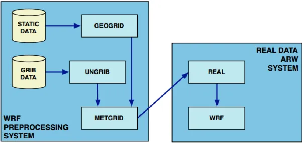
Fig. 17: WRF system components (Skamarock et al. 2008)
Figure 17 shows the principal components of the WRF system, the WRF software framework (WSF) provides the infrastructure that accommodates the dynamics solvers, physics packages that interface with the solvers, programs for initialization, WRF-Var, and WRF-Chem. There are two dynamics solvers in the WSF’ the Advanced Research WRF (ARW) solver and the Nonhydrostatic Mesoscale Model (NMM) solver (Skamarock et al. 2008). 3.3.1. Governing Equations
The ARW dynamics solver integrates the compressible, non-hydrostatic Euler equations. The equations are formulated using a terrain-following hydrostatic-pressure vertical coordinate denoted by 𝜂 and defined as:
( 1 )
𝑝ℎ is the hydrostatis component of the pressure and 𝑝ℎ𝑠 and 𝑝ℎ𝑡 refer to values along the surface and top boundaries respectively. 𝜂 varies from a value of 1 at the surface to 0 at the upper boundary of the model domain, refer to Fig. 18. This vertical coordinate is also called a mass vertical
28 coordinate.
𝜇(𝑥, 𝑦) represents the mass per unit area within the column in the model domain at (𝑥, 𝑦), the appropriate flux form variables are
( 2 ) 𝑉 = (𝑈, 𝑉, 𝑊) are the covariant velocities in the two horizontal and vertical directions, respectively, while 𝜔 = 𝜂 is the contravariant “vertical” velocity. 𝜃 is the potential temperature. Also apperating in the governing equations of the ARW are the non-conserved variables 𝜙 = 𝑔𝑧 (the geopotential), 𝑝 (pressure), and 𝛼 = 1/𝜌 (the inverse density).
Fig. 18: ARW 𝜂 coordinate.
Using these variables definitions, the flux-form Euler equations can be written as:
( 3 ) ( 4 )
29
( 5 ) ( 6 ) ( 7 ) ( 8 ) Along with the diagnostic relation for the inverse density
( 9 ) And the equation of state
( 10 ) In equations 3 and 10, the subscripts x, y and h denote differentiation
( 11 ) and
( 12 ) Where 𝑎 represents a generic variable 𝛾 = 𝑐𝑝/𝑐𝑣=1.4 is the ratio of the heat capacities for dry air, 𝑅𝑑 is the gas constant for dry air, and 𝑝0 is a reference pressure (typically 105). The right hand side terms 𝐹
𝑈, 𝐹𝑉, 𝐹𝑊, and 𝐹Θ represent forcing terms arising from model physics, turbulent mixing, spherical projections, and the earth’s rotation
The prognostic equations 3 to 8 are cast in conservative form except for 8 which is the material derivative of the determination of the geopotential.
Moisture is included by formulating the moist Euler equations, which retain the coupling of dry air mass to the prognostic variables and also retain the conversion equation for dry air (equation 7), In addition the coordinate is defined with respect to the dry air mass, the vertical coordinate can be written as:
30
( 13 )
Where 𝜇𝑑 represents the mass of the dry air in the column and 𝑝𝑑ℎ and 𝑝𝑑ℎ𝑡 represent the hydrostatic pressure of the dry atmosphere and the hydrostatic pressure at the top of the dry atmosphere. The coumpled variables are defined as:
( 14 ) With these definitions, the moist Euler equations can be written as:
( 15 ) ( 16 ) ( 17 ) ( 18 ) ( 19 ) ( 20 ) ( 21 )
With the diagnostic equation for dry inverse density
( 22 ) And the diagnostic relation for the full pressure
( 23 ) Where 𝛼𝑑 is the inverse density of the dry air and 𝛼 is the inverse density taking into account the full parcel density 𝛼 = (1 + 𝑞𝑣 + 𝑞𝑐+ 𝑞𝑣+ ⋯ ) where 𝑞∗ are the mixing rations for water vapor, cloud, rain, ice, etc.
3.3.2. Initial Conditions
31
simulations, or it may be run using interpolated data from either an external analysis or forecast for real-data cases.
The initial conditions for the real-data cases are pre-processed through a separate package called the WRF Preprocessing System. The output from WPS is passed to the real-data pre-processor in the ARW which generates initial and lateral boundary conditions.
3.3.2.1. Reference State
In order to conduct the simulation for real-data conditions the flow in Fig. 19 is required. The flow chart shows the data flow and program components and how it feeds the initial conditions to ARW. The names inside the rectangular boxes are the program’s names, GEOGRID defines the model domain and create static files of terrestrial data, UNGRIB decodes GriB data and METGRID interpolates meteorological data to the model domain.
Fig. 19: Flow chart displaying the data flow and program components for the use of a Reference State for a simulation (Skamarock et al. 2008). The reference state is defined by terrain elevation and three constants: 𝑝𝑜 (105Pa) reference sea level pressure, 𝑇
𝑜 (270 °K – 300 °K) reference sea level temperature, and 𝐴 (50 °K ) temperature difference between the pressure levels of 𝑝𝑜 and 𝑝𝑜/𝑒.
32
With these parameters, the dry reference state surface pressure is given by
( 24 ) From equation 24, the three dimensional reference pressure (dry hydrostatic pressure 𝑝𝑑ℎ) is computed as a function of the vertical coordinate 𝜂 levels and the model top 𝑝𝑑ℎ𝑡:
( 25 ) With equation 25, the reference temperature is defined as
( 26 ) From the reference temperature and pressure, the reference potential temperature is defined as
( 27 ) Then the reciprocal of the reference density using equations 25 and 27 is given by
( 28 ) The base state difference of the dry surface pressure from equation 24 and the model top is given by
( 29 ) From equations 28 and 29, the reference state geopotential defined from the hydrostatic relation is given by
33 3.3.3. Nesting
Fig. 20: 1-way and 2-way nesting options (Skamarock et al. 2008). Nested grid simulations can be produced using either 1-way nesting or 2-way nesting as outlined in Fig. 20. The 1-way and 2-way nesting options refer to how a coarse grid and the fine grid interact. In both the 1-way and 2-way simulation modes, the fine grid boundary conditions are interpolated from the coarse grid forecast. In a 1-way nest, this is the only information exchange between the grids. In the 2-way nest integration, the fine grid solution replaces the coarse grid solution for coarse grid points that lie inside the fine grid. This information exchange between the grids is now in both directions.
34
Fig. 21: Various nest configurations for multiple grids (Skamarock et al. 2008).
Figure 21 displays different nest configurations available. (a) simulation involves one outer grid and may contain multiple inner nested grids.
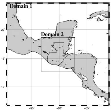
3.4. Computational Conditions
In order to simulate the weather over the Guatemalan territory the computational domains are set as Fig. 22. The domains are nested as indicated in the figure. Table 5 shows the computational conditions. The horizontal resolution of the inner domain, Domain 2 is 10 km. The computation period is the whole one year in 2011. As the initial and boundary conditions for the weather computations, the Final Analysis Data released from the National Center for Environmental Prediction (NCEP) (NCAR Data Support Section, Data for Atmospheric and Geociences Research 2014) is applied.
The NCEP Final Operational Global Analysis data are on 1-degree by 1-degree grids prepared operationally every six hours. The data comes from the Global Data Assimilation System (GDAS), which continuously collects observational data from the Global Telecommunications System (GTS), and other sources. The analyses are available on the surface, at 26 mandatory levels from 1000 millibars to 10 millibars, in the surface boundary layer and at some sigma layers, the tropopause and a few others. Parameters include surface pressure, sea level pressure, geopotential height, temperature, sea surface temperature, soil values, ice cover, relative humidity, u- and v- winds,
35
vertical motion, vorticity and ozone (NCAR Data Support Section, Data for Atmospheric and Geociences Research 2014). The variables included in the NCEP Final Analysis are displayed in Table 4.
Table 4: Variables included in NCEP Final Analysis (NCAR Data Support Section, Data for Atmospheric and Geociences Research 2014)
Air Temperature Clud Liquid
Water/Ice
Convection Evaporation
Geoptential Height Humidity Hydrostatic Pressure
Ice Extent
Land Cover Planetary Boundary Layer Height
Potential Temperature
Precipitable Water Sea Level Pressure Sea Surface
Temperature Skin Temperature Snow Water Equivalent Soild Moisture/Water Content
Soil Temperature Surface Air Temperature
Surface Pressure Surface winds Terrain Elevation Tropopause Tropospheric
Ozone Upper Level Winds Vertical Wind Motion Vorticity
36
Fig. 22: Computational domains for the meteorological model, WRF Table 5: WRF model settings for the evaluation of the weather and
irradiance in Guatemala.
Period Start: 2011/01/01 00:00:00 UTC End: 2012/01/01 00:00:00 UTC
Input Data NCEP final analysis (6-hourly, 1 degree x 1 degree)
Output Data 1-hour interval
Nesting 2-way nesting
Domain Domain 01, D01 (30 km, 61 x 61 grids) Domain 02, D02 (10 km, 61 x 61 grids) Vertical layer 50 levels (surface to 100 hPa)
FDDA option Disable 3.5. Computed Solar Irradiance 3.5.1. Irradiance Maps
Figure 23 shows the global horizontal irradiance (GHI) calculated with WRF. The GHI in this figure is the daily irradiance averaged in the year
37
2011. The irradiance distribution is discussed here with the geography of the country shown in Fig. 3. As it can be seen in Fig. 3, There are two mountain chains south of the 16°N grid line that cross the country from west to east. These areas have low GHI in the mountains (3.5 - 4.5 kWh/m2), and high (5.5 – 7.0 kWh/m2) GHI in the plateaus in the middle of the mountain ranges. North of the 16°N grid line is a flat area with rain forests and high humidity, where GHI is low (4.0 - 5.0 kWh/m2). The southern coast facing the Pacific Ocean has high GHI (6.0 - 7.0 kWh/m2) and is a relatively flat area. Figure 24 shows the yearly GHI in 2011. The irradiance in the high GHI area located in the southern coast reaches almost 2.5 MWh in the year.
Fig. 23: Global horizontal irradiance in Guatemala. Daily irradiance averaged in the year 2011.
Daily average GHI (kWh/m2)
Daily average GHI
38
Fig. 24: Global horizontal irradiance in Guatemala. Yearly in 2011. 3.5.2. Time Series Solar Irradiance
Figure 25 shows the daily GHI averaged in a week at the meteorological station in Guatemala City in 2011 (Instituto Nacional de Sismología, Vulcanología, Meteorología e Hidrología 2014). The station is located in low latitude, the sun passes the zenith at the end of April and the middle of August there. Therefore, if there aren’t are any effects of the weather to the irradiance the GHI should be the largest in these months, the figure shows that the higher irradiance is relatively high in the dry season (from December to the next May), particularly from February to April, and low due to the cloudy and rainy weather of the wet season (from June to November) in particular from August to October. Due to the variations in GHI throughout the year, the daily solar irradiance and also the PV generation is required for the analysis of the grid management in the following section 6. The observed daily GHI averaged in each month is compared between the simulated data with the WRF in Fig. 26. The WRF estimates the GHI is a
39
little larger than the observations. The difference is 8% in average for the daily irradiance. The WRF traces the observed monthly irradiance as shown in Fig. 26.
Fig. 25: Observed daily Global Horizontal Irradiance at the meteorological station in Guatemala City, averaged in a week (Instituto Nacional de Sismología, Vulcanología, Meteorología e Hidrología 2014)
Fig. 26: Daily GHI averaged in each month, evaluated with WRF and observed. (Instituto Nacional de Sismología, Vulcanología, Meteorología e Hidrología 2014) 0 1 2 3 4 5 6 7 8 Ir radi anc e (k W h /m 2) 0 1 2 3 4 5 6 7 8 Ir ra di anc e k W h /m 2
40 3.5.2.1. WRF Irradiance validation
In addition the measurements from selected stations in Guatemala, collected by SUNY, are compared to the WRF. The following graphs (Fig. 27(a) – 27 (n)) compare the 5 years of observed data from the 14 meteorological stations. The meteorological stations used in the study conducted by SUNY are still in operation, however, the instruments for measuring DNI and GHI belonged to SUNY and were removed after they study was finished. The only station that still measures GHI is in Guatemala City and the measurements are compared with the results from WRF in Fig. 26.
Fig. 27 (a): Chiquimula meteorological station, daily global horizontal irradiance Wh/m2 0 1000 2000 3000 4000 5000 6000 7000 8000 9000 1 2 3 4 5 6 7 8 9 10 11 12 Ir radi anc e W h /m 2 Month Chiquimula GHI month average
41
Fig. 27 (b): Cobán meteorological station, daily global horizontal irradiance Wh/m2
Fig. 27 (c): Guatemala City meteorological station, daily global horizontal irradiance Wh/m2 0 1000 2000 3000 4000 5000 6000 7000 1 2 3 4 5 6 7 8 9 10 11 12 Ir radi anc e W h /m 2 Month Cobán
GHI month average
WRF GHI 1998 1999 2000 2001 2002 Average 0 1000 2000 3000 4000 5000 6000 7000 8000 9000 1 2 3 4 5 6 7 8 9 10 11 12 Ir radi anc e W h /m 2 Month Guatemala City GHI month average
42
Fig. 27 (d): Highest Guatemala meteorological station, daily global horizontal irradiance Wh/m2
Fig. 27 (e): Huehuetenango meteorological station, daily global horizontal irradiance Wh/m2 0 1000 2000 3000 4000 5000 6000 7000 8000 9000 1 2 3 4 5 6 7 8 9 10 11 12 Ir radi anc e W h /m 2 Month Highest Guatemala GHI month average
WRF GHI 1998 1999 2000 2001 2002 Average 0 1000 2000 3000 4000 5000 6000 7000 8000 1 2 3 4 5 6 7 8 9 10 11 12 Ir radi anc e W h /m 2 Month Huehuetenango GHI month average
43
Fig. 27 (f): Jalapa meteorological station, daily global horizontal irradiance Wh/m2
Fig. 27 (g): Motagua Valley meteorological station, daily global horizontal irradiance Wh/m2 0 1000 2000 3000 4000 5000 6000 7000 8000 9000 1 2 3 4 5 6 7 8 9 10 11 12 Ir rad ian ce W h /m 2 Month Jalapa
GHI month average
WRF GHI 1998 1999 2000 2001 2002 Average 0 1000 2000 3000 4000 5000 6000 7000 8000 1 2 3 4 5 6 7 8 9 10 11 12 Ir radi anc e W h /m 2 Month Motagua Valley GHI month average
44
Fig. 27 (h): Lowest Guatemala meteorological station, daily global horizontal irradiance Wh/m2
Fig. 27 (i): North Lake Petén meteorological station, daily global horizontal irradiance Wh/m2 0 1000 2000 3000 4000 5000 6000 7000 8000 1 2 3 4 5 6 7 8 9 10 11 12 Ir radi anc e W h /m 2 Month Lowest Guatemala GHI month average
WRF GHI 1998 1999 2000 2001 2002 Average 0 1000 2000 3000 4000 5000 6000 7000 8000 1 2 3 4 5 6 7 8 9 10 11 12 Ir radi anc e W h /m 2 Month North Lake Peten GHI month average
45
Fig. 27 (j): Pacific Coast 1 meteorological station, daily global horizontal irradiance Wh/m2
Fig. 27 (k): Pacific Coast 2 meteorological station, daily global horizontal irradiance Wh/m2 0 1000 2000 3000 4000 5000 6000 7000 8000 1 2 3 4 5 6 7 8 9 10 11 12 Ir radi anc e W h /m 2 Month Pacific Coast 1 GHI month average
WRF GHI 1998 1999 2000 2001 2002 Average 0 1000 2000 3000 4000 5000 6000 7000 8000 9000 1 2 3 4 5 6 7 8 9 10 11 12 Ir radi anc e W h /m 2 Month Pacific Coast 2 GHI month ave
46
Fig. 27 (l): Puerto Barrios meteorological station, daily global horizontal irradiance Wh/m2
Fig.27 (m): Quetzaltenango meteorological station, daily global horizontal irradiance Wh/m2 0 1000 2000 3000 4000 5000 6000 7000 8000 1 2 3 4 5 6 7 8 9 10 11 12 Ir radi anc e W h /m 2 Month Puerto Barrios GHI month average
WRF GHI 1998 1999 2000 2001 2002 Average 0 1000 2000 3000 4000 5000 6000 7000 8000 1 2 3 4 5 6 7 8 9 10 11 12 Ir radi anc e W h /m 2 Month Quetzaltenango GHI month average
47
Fig. 27 (n): Retalhuleu meteorological station, daily global horizontal irradiance Wh/m2
For each station a statistical comparison between the GHI obtained from WRF and the 5 year average is conducted. This statistical comparison consists in a 2 sample T test for comparison of the means, and an F test to compare the variances and determine if the 2 samples are statistically equal. The results are summarized in Table 6.
Table 6: Meteorological Stations, statistical tests results 2 Sample t Test and F Test with 95% Confidence Level
Meteorological Station
2 Sample t Test F Test Test Value Critical Value Test Value Critical Value Chiquimula 0.54 2.45 2.4 2.82 Cobán -1.19 2.45 3.42 2.82 Guatemala 0.57 2.45 2.02 2.82 Highest Guatemala 0.71 2.45 1.59 2.82 0 1000 2000 3000 4000 5000 6000 7000 1 2 3 4 5 6 7 8 9 10 11 12 Ir radi anc e W h /m 2 Month Retalhuleu GHI month average
48
Huehuetenango -0.14 2.45 1.37 2.82
Jalapa 0.69 2.41 1.38 2.82
Lowest Guatemala -1.19 2.41 2.82 2.82
Motagua Valley -0.46 2.42 2.16 2.82
North Lake Petén -1.01 2.45 2.52 2.82
Quetzaltenango -1.95 2.41 1.08 2.82
Pacific Coast 1 2.23 2.41 1.47 2.82
Pacific Coast 2 2.04 2.42 1.78 2.82
Puerto Barrios 0.39 2.42 1.83 2.82
Retalhuleu 0.15 2.41 2.05 2.82
The statistical tests indicate that the calculated GHI from WRF and the measurements from the different stations have equal means and variances with confidence level of 95%.The only station that does not fit is Cobán, which the F test result indicate that the variances of the WRF GHI and the observed GHI are not equal. The results indicate that the WRF data presents equal means and variances for most of the cases and therefore it can be used for the present research. In addition the distribution maps created using WRF GHI were compared with Figures 13, 14 and 15 they display similar distribution and further validate the WRF GHI. However the WRF GHI distribution has higher resolution (10km by 10km) than Fig. 13 and Fig. 14 (40km by 40km) and it also provides the time series with a one hour interval instead of the average GHI provided in Figures 13, 14 and 15.
49 4. PV Output in Guatemala
4.1. PV Output Estimation
In the previous sections some meteorological parameters, including global horizontal irradiance (GHI) and ambient temperature, in Guatemala are evaluated by using the meteorological model WRF. The output of a PV system is estimated in this section from the meteorological parameters.
There are many PV panel types in these days. The installation of crystalline silicon photovoltaic panels is assumed here, because they are one of the most popular panel types in these days. The crystalline silicon photovoltaic cells account for roughly 80% to 85% of the global production according to the U.S. Solar Photovoltaic Manufacturing Industry Trends, Global Competition, Federal Support report (Platzer 2012).
Huld, et al. (2011) proposes the following equation to evaluate PV output, P(G',T') for the general crystalline silicon photovoltaic panels.
𝑃(𝐺′, 𝑇′) = 𝐺′(𝑃
𝑆𝑇𝐶,𝑚+ 𝑘1ln(𝐺′) + 𝑘2ln(𝐺′)2 +𝑘3𝑇′+ 𝑘
4𝑇′ln(𝐺′) + 𝑘5𝑇′ln(𝐺′)2+ 𝑘6𝑇′2) ( 31 ) Where G' is the normalized in-plane irradiance, and is computed by dividing by the in-plane irradiance G by 1,000 W/m2. T' is the temperature of the module measured on the standard test conditions. PSTC,m is the power rating of the module; in this Part 1, 1 kW power rating is assumed for the module. The six constants 𝑘1 to 𝑘6 were derived empirically from the indoor experiment conducted by these authors and are displayed in Table 7.
50
Table 7: constants 𝑘1 to 𝑘6 from Huld el al. 2011. Constants Values and dimensions
𝒌𝟏 −0.01724(𝑑𝑖𝑚𝑒𝑛𝑠𝑖𝑜𝑛𝑙𝑒𝑠𝑠) 𝒌𝟐 −0.04047(𝑑𝑖𝑚𝑒𝑛𝑠𝑖𝑜𝑛𝑙𝑒𝑠𝑠) 𝒌𝟑 −0.0047(°𝐶−1) 𝒌𝟒 1.49 × 10⁻⁴(°𝐶−1) 𝒌𝟓 1.47 × 110−4(°𝐶−1) 𝒌𝟔 5.0 × 110−6(°𝐶−2)
The in-plane irradiance G, that reaches the plane with tilted angle β is estimated with the following the model proposed by Duffie and Beckman’s (2006);
𝐺 = 𝐵ℎ𝑅𝑏(𝛽) + 𝐷ℎ𝑅𝑑(𝛽) + 𝐺𝑔𝜌𝑅𝑟 ( 32 )
Where Bh is the direct normal irradiance on the horizontal plane. Dh and Gg are the diffused and the global horizontal irradiance, respectively. Rb(𝛽), Rd(𝛽) and Rr are the transposition factors for the direct, the diffused and the reflected irradiance, respectively. ρ is the albedo of the ground.
In this study, the ground reflected irradiance is assumed isotropic, and the following equation (Duffie and Beckman 2006) is applied:
𝑅𝑟 = (1 − cos 𝛽) 2⁄ ( 33 )
The albedo ρ varies depending on the surface type and its conditions. Kambezidis, Psiloglou and Gueymard (1994) found that the anisotropic albedo models do not improve the estimation for the solar irradiance on south oriented surfaces,therefore a fixed albedo is used here. A general value of 0.3 is used for the albedo according to Ahrens (2009) since the country is mostly covered in forests and grasslands.
Padovan and Del Col (2010) tested some models available for the estimation of diffused irradiance on the horizontal and tilted planes. They
51
reported that the models proposed by Liu and Jordan (1963), Klucher, (1979), Perez et al. (1990) and Reindl et al. (1990) estimate the diffuse irradiance with similar accuracy. The transposition factor for the diffuse irradiance on the plane Rd(β) is estimated by using the following equation proposed by Liu and Jordan (1963) is applied:
𝑅𝑑(𝛽) = (1 + cos 𝛽) 2⁄ ( 34 )
Direct irradiance is estimated by Duffie and Beckman (2006) model, which describes the transposition factor for direct irradiance on the plane 𝑅𝑏(𝛽) as;
𝑅𝑏(𝛽) = cos 𝜃𝛽⁄cos 𝜃 ( 35 )
Where 𝜃𝛽 and 𝜃 are the solar incidence angles on the plane with the tilted angle 𝛽 and on the horizontal plane, respectively.
The direct and diffused irradiances are estimated by the GHI computed with WRF, and the above models.
Several models to evaluate the direct and diffused irradiances are proposed. And they are analyzed and compared by Khalil and Shaffie (2013). They reported that for south facing surfaces, the models proposed by Perez, et al. (1987), Skartveit, et al. (1987) and Hay (1979) have the most accurate predictions with the similar accuracy. Therefore the model proposed by Skartveit, et al. (1987) was chosen in this paper. It is indicated as follows; For 𝐺𝑔⁄𝐺0 ≤ 0.22 𝑟𝐷 = 1.0 − 0.09(𝐺𝑔⁄ ) 𝐺0 ( 36 ) For 0.22<Gg⁄G0≤0.80 𝑟𝐷 = 0.951 − 0.1604(𝐺𝑔⁄ ) + 4.388(𝐺𝐺0 𝑔⁄ )𝐺0 2 −16.638(𝐺𝑔⁄ )𝐺0 3 + 12.336(𝐺𝑔⁄ )𝐺0 4 ( 37 )
52 For 𝐺𝑔⁄𝐺0 > 0.80
𝑟𝐷 = 0.165 ( 38 )
𝐷ℎ = 𝐺𝑔 × 𝑟𝐷 ( 39 )
𝐵ℎ = 𝐺𝑔× 1 𝑟⁄ 𝐷 ( 40 )
Where G0 is the Solar Constant and rD is an empirical parameter estimated by Skartveit and Olseth (1987) in order to calculate the diffuse and the direct components of the GHI.
Huld, et al. (2011) also proposes the empirical model to evaluate the module temperature T' under standard test conditions from the ambient
temperature Tamb and the in-plane irradiance 𝐺 as follows: 𝑇′= 𝑇
𝑚𝑜𝑑− 25℃ ( 41 )
𝑇𝑚𝑜𝑑 = 𝑇𝑎𝑚𝑏+ 𝑘𝑇𝐺 ( 42 )
Where Tmod is the temperature of the module, Tamb is the ambient temperature and kT is a constant related to the panel type and G is the in-plane irradiance. The typical values of this constant range from 0.03 to 0.035 °Cm2W-1. This study uses the value 0.035 °Cm2W-1, which is the same one used in Huld et al (2011). Their results from the indoor experiment also showed that Eq. 31 predicts the PV output within 1% error. However, for irradiances lower than 100 W/m2 the predictions fit within 5% to 10% error (Huld et al. 2011).
4.2. PV Generation and Tilted Angle
In order to determine the optimal tilted angle for PV panels in Guatemala, the energy productions are evaluated with different tilted angles from 0° to 30°, with a 1 kW installed PV capacity. The target site chosen for this analysis is Guatemala City (14°35’14” N, 90°31’59”W), which is located in the middle of the country as shown in Fig. 3.
53
the PV energy output. It shows that the energy production increases moderately from 0° until reaching its peak at 10°. Afterwards the energy production drops, as the angle becomes larger. From this figure, the angle 10° is lead as the optimal tilted angle for the solar panels in the target point.
Fig. 28: PV output in relationship with tilted angle of a panel (Power rating 1 kW, facing to south)
4.3. Energy Potential Maps
The output of the PV system is evaluated in Guatemala with the methods explained above, and it is indicated as the PV potential map as shown in Fig. 29. The tilted angle of the PV panels is assumed to be 10°, which is the optimal tilted angle in Guatemala City derived in the previous section. The map shows that the estimated total PV output for one year in Guatemala generated from the PV system with a power rating 1 kW.
1.96 1.98 2 2.02 2.04 2.06 2.08 0 5 10 15 20 25 30 35 Y ea rl y P V O u tp ut (M W h ) Tilted Angle