Strategies for an Optimized simulation of granular particles in a Newtonian Fluid, Part 1: Basics(Mathematical Aspects of Complex Fluids and Their Applications)

Strategies

for

an

Optimized

simulation

of

granular

particles

in

a

Newtonian

Fluid,

Part 1:

Basics

Hans-Georg Matuttis,

University ofElectro-Communications, Department ofMechanical Engineeringand

Intelligent Systems, Chofu, Chofugaoka 1-5-1, Tokyo 182-8585 Japan

Abstract; _In this article,

an

outline is given for an an “ideal” simulation of

granular particles in fluids with respect to CPU-effort, accuracy etc. which

features should be incorporated in the underlying simulation, and which

nu-merical techniques should be used with respect to the time integration.

1

Introduction

Though many features of granular materials , especially those in connection with static

or

quasi-static regimes (heap-formation, arching), awhole class or granular phenomena is

influenced by the surrounding fluid:

Fluidized beds and Sedimentation are the terms used to describe systemswhere

grains in various concentrations interact with the surrounding fluid under the influence

of gravity.

Pattern formation processes like rippling and dune formation take place in in air

and under water. Hydrological phenomenalike the formation ofcoastlines, the formation

and destruction of river banks and and the changeof river beds also belongs in this class.

Dust avalanches of powder snow, where the avalanche is supposed to ride on a

cushion of compressed air, are much faster, far reaching and

more

destructive than the

fluid-tike avalanches of ”sherbet-like” snow,

Pneumatic transport is the field which deals with the intentional or unintentional

movement of granular materials by fluids, ranging from

vacuum

cleaners over devices in

$\mathrm{c}\mathrm{h}\mathrm{e}$mical engineering to sandstorm $\mathrm{f},,$.

Porous Media is the field where the surrounding”granular matrix” is considered to

be stationary, and only the fluid it contains in the pore space is supposed to

mover

Landslides

are

the result of an interaction between

a

granulaJ matrix of a slopeand

a pore fluid which destabilizes the whole system.

We will outline which features must be

incorpo-rated in a simulation to

access

the widest range of

the above phenomena with the minim um amount of

computational effort while retaining physical

valid-ity. The granular materials shall be modeled on the

particle level (Lagrangian method), to be able to

in-vestigate micro-mechanicmechanisms ofmacroscopic

phenomena. The surrounding fluid should be simu- Figure 1: Grid artifact: Though

latedin agrid-based discretization

as

Newtonian fluid the relativepositionof particle Pi

(Eulerian method),

so

that artifacts introduced by versu$\mathrm{s}$ P2 is the

same

as

that of

some

grid-based methods (Lattice-Gas automata[9], particle P3

versus

P4, in the first

Lattice Boltzmann simulations$[6, 17]$_, see _Fig.1)

are case

the path between the

parti-avoided. Particle based methods (moving particle cles is blocked, only in the latter

sem i-im plicitMPS$[16, 15]$_{, smoothedparticle dynam-} case there is a pathfor the fluid,

1. it allows the input of realistic conditions (particle shape, friction, etc),

2. is able to reproduce themacroscopic (rippling,

. .

.) and mesoscopic (saltation, collapse

of fluid-filled cavities,

. .

) behavior,

3.

can

be used for low (sedimentation) and high (porous media) granular density alike,

4. uses the ninimurn amount of computer time and storage in comparison with other

com putational methods and

5. maybe iseven faster (in realtime) than apurely “dry” simulationor a pure liquiddue

to a-prioriconsiderations which will be explained below.

Previous simulations have dealt with the incorporation of particles into

a

fluid by

usinga straightforward approach, usingthe standard square grid with MAC[12] (marker

and cell) and the standard granularparticle simulation with round particles. Apart from thle problemthat the blocking of flow by particles cannot be treated with round particles,

most of the algorithmic effort went into the treatment of the incomm ensurability of the

straight grids and curved grain boundaries. Kajishima[14] used a brute-force approach, putting sub-meshes around the particles several orders of magnitude smaller than the

particle diam etcr; the accuracy gained in the description of the particle outline lead to a

huge blowup of the number of mesh-points, and accordingly, the CPU-effort is gigantic.

Schwarzeret $\mathrm{a}1[29.,$13,30] tried to match the particleswith asirriilar-sizedmesh, coupling

the particle motion to tracer particles in the fluid: In a sense, the fluid goes “through”

the particle, which

are

$’\backslash \mathrm{f}\mathrm{i}\mathrm{x}\mathrm{e}\mathrm{d}^{\backslash }$’ to the flow lines

with “springs”. These ”

$\mathrm{s}\mathrm{p}\mathrm{r}\mathrm{i}\mathrm{n}\mathrm{g}\mathrm{s}’\backslash$

(cou-pling constants) introduce additional degrees of freedom (stiffness, damping), for which

the timescale is difficult to predict, which leads to numerically instable choices of the

time-step. Moreover, most of the Computer time (99

%)

goes in the solution of the

MAC-pressure-iterationfor the incompressibility-condition, due to incommensurability of

particle boundaries and grid positions. In this article, we will explain how to circumvent

the above problems by not choosing the most straightforward approach in the

model-ing of the primitives of the simulation (round particles, quadrilateral grid), but with tlie

advantageth at the treated ent of the particle-fluid interface becomes straightforward.

1.1

$\mathrm{C}\mathrm{o}\mathrm{n}\mathrm{t}\mathrm{i}\mathrm{n}\mathrm{u}\mathrm{u}\mathrm{m}/$

Fluid

part

The sound velocity $c$ of a continuum solid

can

be calculated from its Young modulus $Y$

and its density $\rho$as $c=\sqrt{Y/\rho}$Thesound velocity ofa chain made ofspherical particlesis

about 10 % of that of the continuum material the particles

are

madeof: $c_{chain}\approx 0.1\mathrm{c}$. The

sound velocity of a th ee-dim ensional disordered packing of mono-disperse particles $c_{\mathrm{d}\mathrm{j}\mathrm{s}}$

is again

on

order ofmagnitude less,

so

that the relation $c_{\mathrm{d}}\mathrm{i}\mathrm{s}$ $\approx 0.\mathrm{l}\mathrm{c}\mathrm{c}\mathrm{h}\mathrm{a}\mathrm{i}\mathrm{n}\approx 0.0\mathrm{l}\mathrm{c}$hold[25].

Therefore, the sound velocity of thegranular part

can

be considered considerably lower

than that of the fluid part, which itselfisabout that ofacontinuumsolid. Therefore, the

fluid part will be best approxim ated as an incompressible fluid. If,

as

a starting point,

the fluid is to be approximated

as

a Newtonian fluid, this

means

that the incompressible

(a) Spherical smooth glass (b) Smooth non-spherical (c) Rough,“crushed” glass

beads beads

Figure 2: Effect ofelongation and surface structure ofglass beads on the critical angle

1.2

Particle Modeling

The bulk properties of assemblies of circular $/\mathrm{s}\mathrm{p}\mathrm{h}\mathrm{e}\mathrm{r}\mathrm{i}\mathrm{c}\mathrm{a}\mathrm{l}$ granularparticles differ

consider-ably from that of non-spherical particles: Whereas the angle of repose for dry spherical

glass beads in Fig. $2(\mathrm{a})$ is about 20 degrees, if “straight” slopes can be identified at all,

for the elongatednon-sphericalparticles in Fig.$2(\mathrm{b})$oneobtains a more sand-like angleof

repose of about 30 degrees. Surface roughness of the grains and the size dispersion

rela-tion alsoeffects the angle of repose, as the angle of reposefor the rough glass’s in Fig.$2(\mathrm{c})$

shows. Anotherquantitativedifference

can

beseenin thestress-strain diagram,where the maximal yield strength of elongated polydisperse particles is twice that of round particles

(Fig.$3(\mathrm{a})$)

$)$ and the differences in the density-strain diagram also shows that the internal

structure must be different (Fig.$3(\mathrm{b})$). For these reasons, a simulation ofgranular

parti-cles in

a

fluid should make

use

of non-spherical particles, so that e.g. for sedim entation,

the resulting slopescan be computed with acceptablestability and precision.

$\mathrm{J}\Omega\underline{\underline{0\alpha(n}}$

(a) Stress-strain,scaled by the external pres- (b) Density-strainscaled bythe density

be-fore$\mathrm{c}\mathrm{o}$mpression $\mathrm{i}>\iota\iota \mathrm{r}\mathrm{e}$

Figure 3: Granular properties of

a

typical single run of biaxial compression of

mono-disperse round particles (full line), polydisperse round particles (dashed line) and

poly-disperse elongated particles (dotted line) [21].

springmodel [7]

or

the numericalexactimplementation

(”Conctact dynamics”$\mathrm{c}\mathrm{i}\mathrm{t}\mathrm{e}\mathrm{m}\mathrm{o}\mathrm{r}\mathrm{e}\mathrm{a}\mathrm{u}88,\mathrm{m}\mathrm{o}\mathrm{r}\mathrm{e}\mathrm{a}\mathrm{u}89$, or Ref.$\mathrm{c}\mathrm{i}\mathrm{t}\mathrm{e}\mathrm{H}\mathrm{a}\mathrm{i}\mathrm{r}\mathrm{e}\mathrm{r}:93$, p.199) is used : This

excludes the possibility ofmodeling the particles with elliptic potentials[32], which gives

only

a

force direction, but not a traceable contact point. All in all, the use of

polygo-nal (polyhedral in three dimensions) particles in connection with a surrounding fluid is

preferable to e.g. particles with curved boundaries, because the geometric information is

geometrically better defined.

Finally, the use of soft particle models (with finite young modulus) is preferable over

“rigidparticles” (infiniteyoung modulus) in event-drivenparticle simutations$[19, 20]$ orin

contact mechanics$[23, 24]$: Event-driven simulations allow only the simulation of binary

collisions, and as there is a suspicion that the net interaction of particles submerged

under wateris attractive, this would disturb agglomeration. Contact mechanicscantreat

multiplecontact (at considerablelarger algorithmiceffort than the event-drivenmethod);

Adrawback is that modeling the granularparticleswith rigidcontactsresults in

an

infinite

soundvelocity,which is physically dubious and in the presence of

an

incompressiblefluids

may lead to serious numerical instabilities due to thhe interference of two infinite signal

velocities.

1.3

Statistical Physics

In accuracy benchmarks in fluid mechanics, e.g. the flow behind an obstacle, “idealized”

boundary conditions for thelikewiseidealizedNewtonianfluidarechosensothat solutions

can

begivenor at least definedinarbitrary precision; in the

case

of Karmanvortices, this

will be an ideal circle or sphere as obstacle. For low Reynolds numbers, this will be the

flow lines, for higher Reynoldsnumbers, where no stationarysolutionexists, one

can

still

expect the existence ofprobabilitydistributions for e.g the size of vortices in the Karman

vortex street which should be reproduced exactly by simulations and experiments alike.

Physically, the relevance of such definitions may be actually doubtful, as experimentally

already for Reynolds numbers

as

low as 20, huge deviations have been found in the

streamlines of flow through a small orifice for polar and non-polar-simulations, on the

one

hand, and the numerical practically exact simulation on the other hand ([31] and

References therein); A-priory, it is unclear why the experimentally used fluids (distilled

water, ethanol and liquid paraffin) deviate sostrongly from ideal Newtonian behavior.

In granular material research from thepoint ofstatisticalphysics,

on

the otherhand,

one is not so much interested in single particle problems with arbitrary precision, but

tries to derive the macroscopic quantities based on the microscopic mechanisms. In that

respect,for the sedimentation of granular particles ina fluid, the experimentalverification

should not bea verification of the particle trajectory (impossible, because it is obviously

a nonlinear-chaotic problem), but the speed ofthe sedimentation fronts, and the angle of

theresulting slopes.

Whereas, as discussed in the previous paragraph, “high accuracy” is not an issue due

costs: No fluctuating noise terms due to lack ofprecision in the solution of the continuity equation should be introduced, because they might lead to unphysicallyoscillatory force

laws, sothat the granular phase would become fiuidized morethan is physically realistic.

Figure 4: Delaunay-Triangulation$\mathrm{s}$ of a square-grid deformed with Gaussian-distributed

random numbers ($\sigma=0/Fr\mathrm{i}edr\mathrm{i}chs-K$eller- Grid, 0.05, 0.1,0.2 )

1.4

The

Grid

Structured grids have the advantage that the resulting system ofequation is

character-ized byaband Matrix,

so

that conventional LU-Solvers canbe used. Thedisadvantage is

that for complicated simulationgeometries, the construction of the grid is

an

arbitrarily

complex task, even

more

soif the neighborhood relation ofthe gridpointsmust be taken

into account as an additional constraint. If two granular particles approach each other,

the space between them can become arbitrarily narrow: The treatment of the fluid with

a

more or

less uniform grid spacing, as prevalent inthe MAC-method, isnot suitable for

this case, because if the regular grid with the smallest gridsize (smallest particledistance)

is used, this leads tounnecessary manydegrees offreedom.

Unstructured gridsgivethe largest freedom for the distribution of themesh-points,

andcantherefore be optimally adaptedtothe particle- and flow-geometry. The

disadvan-tage isthat “numerically exact” LU-Solvers becomeinefficient, ad sparsematrixmethods

have to employed, which

are

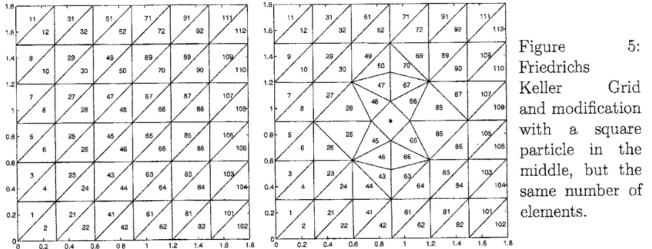
numerically considerably less stable.

Figure 5: Friedrichs Keller Grid and modification with a square particle in the

middle, but the

same

number of

elements.

To simulate polygonalparticles with a shape-matching grid, triangular elements

gen-erated via Delaunay triangulation will be easier to handle than quadrilateral elem ents,

There is a philosophy in fluid dynamics of immersed bodies which tries to to retain a rectangular grid structure for the fluid simulation at all costs, but introduce the

inter-faces between the fluid and the particle surface with computer science techniques (Ghost

Fluid method, CIP/Multi-Moment,MARS, Level Set method). We refrain from

imple-menting such methods, because each additional interface in a medium introduces a new wave $\mathrm{r}\mathrm{e}\mathrm{s}\mathrm{i}\mathrm{s}\mathrm{t}\mathrm{a}\mathrm{n}\mathrm{c}\mathrm{e}/$ mechanicalimpedance for the signal-

or

momentum-propagation in that

medium, and the scattering properties of the above interfaces are far from clear: In the

worst caseh it _rna7

serve as

a

source

of noise which prevents the build-up of static

con-figurations. Instead, particles form$\mathrm{n}$ the boundaries of the fluid (see Fig.1.4), and the

additional, unphysical degrees of freedom are a nuisance anyway because they increase

the computational complexity and the CPU-time alike. Chimera-Grids are popuiar for

si nulations of few particles ofcomplicated shape inside a fluid, e.g. for the cross-section

of wings, usually in connection with quadrilateral grids; due to

our

choice of granular

particles as polygons and the flexibility ofthe finite element method, the implementation

ofChimera Grids or finer meshes is not necessary

1.5

Discretization

Schemes for the fluid

For the grid part of the simulation, thle algorithm with the least degrees of freedom is

desirable: The leastcom putation effort for lattice methods (PartialDifferential Equations,

Lattice fermions .. ) for $N$ lattice points

can

in som $\mathrm{e}$ cases be obtained for a single

timestep within $N\log N$ operations (if Fourier-Type methods

can

be employed), more

realistic for general problems is a cost of $N^{2}$ operations per timestep. Therefore, the

number ofgrid points should be reduced as much

as

possible. This

can

be accomplished

by using larger meshes with higher-order discretization methods and by choosing the

particle boundary as boundary of the fluid,

so

that the corresponding grid points are

determined by the $\mathrm{g}\mathrm{r}\epsilon‘ \mathrm{L}\mathrm{I}\mathrm{l}\mathrm{u}\mathrm{l}\mathrm{a}\mathrm{r}$ simulation, and inputted as boundary conditions into the

fluid part of the simulation.

Finite Differences have the advantage of being ”simple”, in the

sense

that the

discretized equations still resemble the original differential equations. The disadvantage

is that they work best (”computationa1 most efficient”) for rectangular grids, which

don’t work wellwith the polygonal particles we want to use.

TheFinite Volume method has problems with strongly varying meshsizes, and also

maybe with topological changes of the grid. The whole formalism is considerably metre

complicated than the finite difference method.

The Galerkin Finite Element Method (GFEM) is, ascomplicatedas finite volume

method (but not more so,

as

has been argued in Ref. [26]): it uses the weak form of the

PDE, which

means

thatnot the originaldifferentialequationsare approximated, buttheir

integral This leads to

more

benign behavior for strongly varying solutions (the integral

over a non-differentiable funciton is likely to be differentiable), but it also introduces

additionaldegressoffreedom (oscillatorysolutions additionally to the advective solutions

versatile method for complicated boundaries and unstructured meshes, we will base our

simulation of granular particles in fluids onthis method. The Navier-Stokes equations in

the “strong formulation” can bewritten as

$\frac{\partial u}{\partial t}=-\frac{\partial(u^{2})}{\partial x}-\frac{\partial(uv)}{\partial y}-\frac{\partial\phi}{\partial x}+f_{x}+\iota/(\frac{\partial^{2}u}{\partial x^{2}}+\frac{\partial^{2}u}{\partial y^{2}})$ (1)

$\frac{\partial v}{\partial t}=-\frac{\partial(vu)}{\partial x}-\frac{\partial(v^{2})}{\partial y}-\frac{\partial\phi}{\partial y}+f_{y}+"(\frac{\partial^{2}v}{\partial x^{2}}+\frac{\partial^{2}v}{\partial y^{2}})$ (2)

$0= \frac{\partial u}{\partial x}+\frac{\partial v}{\partial y}$ (3)

with the pressure fields $p$, and the velocity field $u$,$v$ for the flow in $\mathrm{x}/\mathrm{y}$ direction, and

with dynamic viscosity $l/$. The last equation, $\mathrm{e}\mathrm{q}\mathrm{n},3$, the ”continuity equation”,

assures

the incompressibility. as in the “weak formulation”,, the equations have been integrated

over

with basis functions (for $\mathrm{f}\mathrm{i}\mathrm{r}\mathrm{s}\mathrm{t}/\mathrm{s}\mathrm{e}\mathrm{c}\mathrm{o}\mathrm{n}\mathrm{d}$ order finite elements, with polynomials of

$\mathrm{f}\mathrm{i}\mathrm{r}\mathrm{s}\mathrm{t}/\mathrm{s}\mathrm{e}\mathrm{c}\mathrm{o}\mathrm{n}\mathrm{d}$ order respectively) and then integrated out;

$\int\phi(\frac{\partial u}{\partial t})=\int\phi(-\frac{\partial(u^{2})}{\partial x}-\frac{\partial(uv)}{\partial y}-\frac{\partial\phi}{\partial x}+f_{x}+\iota/(\frac{\partial^{2}u}{\partial x^{2}}+\frac{\partial^{2}u}{\partial y^{2}}))$ (4)

$\int\phi(\frac{\partial v}{\partial t})=\int\phi(-\frac{\partial(vu)}{\partial x}-\frac{\partial(v^{2})}{\partial y}-\frac{\partial\phi}{\partial y}+f_{y},[perp]\iota/(\frac{\partial^{2}v}{\partial x^{2}}+\frac{\partial^{2}v}{\partial y^{2}}))$ (5)

$0= \int\phi(\frac{\partial u}{\partial x}+\frac{\partial v}{\partial y})$ $\backslash (6)$

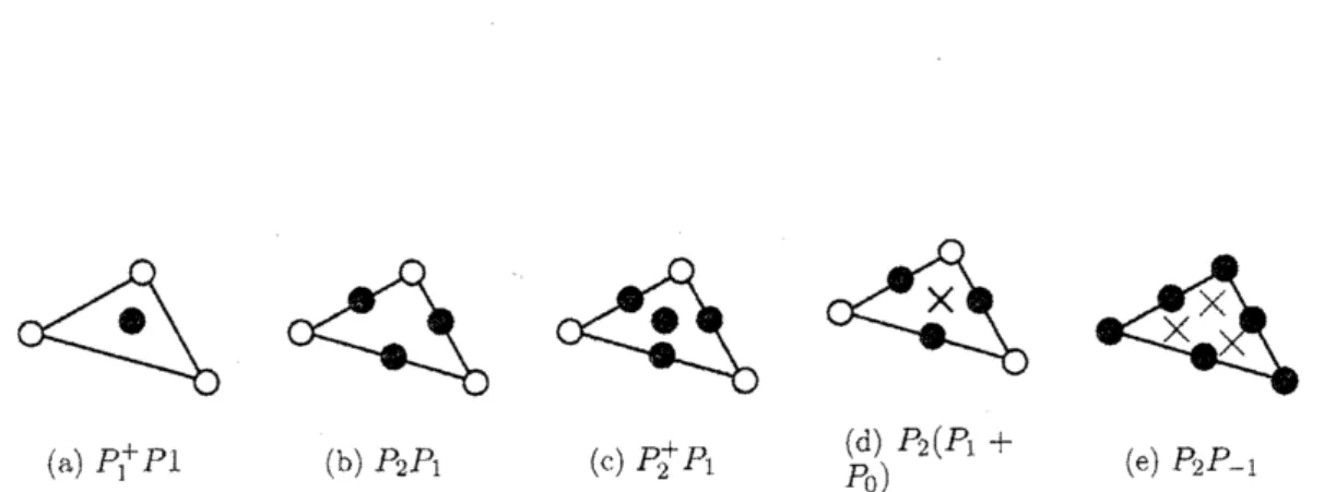
Thereis considerable freedom in thechoiceofelements, i.e. which pointson agrid should

be integrated out, and in which order the approximation should be performed, as can

be seen in Fig.6. Nowadays, there is a $\mathrm{c}\mathrm{o}\mathrm{n}\mathrm{s}\mathrm{e}\mathrm{n}\mathrm{s}\mathrm{u}\mathrm{s}[27_{\rfloor}^{\rceil}$ that because the Navier-Stokes equation is ofsecond order in velocity and first order in pressure, the approximation for

thevelocities should be one order higher than for the pressure, which at least eliminates

the $P_{1}^{+}P1$-element (first order in velocity, first order in pressure) in Fig.$6(\mathrm{a})$. This still

leaves considerable freedom for second order elements. Because $P_{2}(P_{1}+\mathrm{p}_{\mathrm{q}})$

conserves

the element mass, we expect problems due to the volume change of elements induced

by moving boundaries (granular particles), so we will not

use

this element. The $P_{2}P_{-1}$

-element has no pressurepoints onthe element boundaries, so that

no

forces on granular

particles which act

as

element boundaries

can

be computed, so the

use

of th is element

is also excluded. This leaves basically $P_{2}^{+}P_{1}$ and $P_{2}P_{1}$, the latter being simplest second

order element, whichwe will choose for our implementation.

2

Time Integration

2.1

Time consumption

Meaningful criteria for “the fastest algorithms” are not easy to

come

by. In the field

of onte-Carlo simulations, ”updates per second” (UPS) are a common criterion, albeit

not a very meaningful one: Different updating methods come at different computational

{$\mathrm{a})$ $P_{1}^{+}P1$ (b) PfPl (c) $P_{2}^{+}P_{1}$ (e) $P_{2}P_{-1}$

(d) $P_{2}(P_{1}+$

$P_{0})$

Figure6: Various elements for fluid flow where $0$ indicatescontinuousvelocities and

con-tinuous pressures, $\bullet$ indicates continuous velocities and ix indicates discontinuous

pres-sures.

UPS, divided by the half-life time $\tau$ which characterizes the relaxation time. Likewise,

for ordinary differential equations, some time integration methods are more costly per time-step, thanothers, _{e.g. ingeneral implicit} Runge-Kutta methodsare morecostly than

explicit Runge-Kuttamethods. though implicit predictorcorrectormethods ($\mathrm{G}\mathrm{e}\mathrm{a}\mathrm{r}/$

Back-ward $\mathrm{D}\mathrm{i}\mathrm{f}\mathrm{f}\mathrm{e}\mathrm{r}\mathrm{e}\mathrm{n}\mathrm{c}\mathrm{e}/\mathrm{B}\mathrm{D}\mathrm{F}$)

are

not necessarily more costly than explicit (Adams-Bashforth)

methods. Higher order Runge-Kutta (RK) methods are

more

costly than lower

meth-ods because they need more function evaluations per timestep than lower order

meth-ods (n-th order methods RK methods need at least $\mathrm{n}$ function evaluations), whereas for

Predictor-Corrector methods usually a single function evaluation per time step is

suffi-cient. $.\backslash \mathrm{I}\mathrm{e}\mathrm{v}\mathrm{e}\mathrm{r}\mathrm{t}\mathrm{h}\mathrm{e}1\mathrm{e}\mathrm{f}^{\backslash },\mathrm{b}$, the decisive factor is the maximal size of the time step $dt_{\mathrm{r}\mathrm{n}\mathrm{a}\mathrm{x}}$ (called

“radius of stability” in the numerical literature) which

can

be used, so that a meaningful

criterion for the fastest integratoris thethe largest possible timestep for agiven problem

$dt,$, divided by the number of necessary function evaluations. For particles of

mass

$m\epsilon \mathrm{x}t\mathrm{n}\mathrm{d}$

Young modulus $Y$, the characteristic frequency of the corresponding undamped harmonic

oscillatoris$\omega$ $=\sqrt{Y/rr\iota}$. That 1eans that

over

awide range ofvelocities, the contact time

$T$ for

a

single collision

can

be approxim ated well as $T=2\pi/\omega$. Wc have found that for

suitable integrators (Gear-Predictor-Corrector/BDF). the timestep $dt_{1\mathrm{n}\mathrm{a}\mathrm{x}}$

can

be chosen

of the order of$dt\approx T/10$. For particles in

a

fluid, themotion isadditionally damped: Thle

contact time becomes larger and larger time steps

seem

possible. Under the assumptions

that the surfaces and the motiongranular particleserase vortices of small$\mathrm{d}\mathrm{i}\mathrm{a}\mathrm{m}\mathrm{e}\mathrm{t}\mathrm{e}\mathrm{r}/$ small

$\mathrm{t}\mathrm{i}$ me scale, larger grid sizes and larger time steps

seem

possible for the fluid part of the

simulation than for the simulation without particles.

2.2

Method of

Lines

Thediscretization 1n thetime direction will not bedone by finite elements with a

compo-nent in the time domain but with the method of lines[28], i.e. the partial time derivative

is treated as an ordinary derivative, and the solution

can

then be obtained with

conven-tional ordinary differential equation solvers, making use of the substantial theory with

respect to accuracy and stability of that field[ll, 8]. For the simulation of partial

dif-ferential equations with explicit integrators (linearization ofthe time evolution), the size

of the maximal timestep is usually proportional to the lattice spacing. This criterion

based

on von

Neuman stability analysis (linearization of the time evolution operator for

each eigenmode) is usually not valid for implicit integrators, which

are

derived without

2,3

_Relaxation

vs.

_{”numerically exact” methods}

In the MAC-method, the time integration is performed without taking the

incompress-ibility into account. Instead, at the new time step, the velocity is equilibrated with the relaxation condition

$v^{n+1,k+2}=v^{n+1,k+1}-\delta t\nabla(p^{n+1,k+1}-p^{n+1,k})$ ,$k\geq 0$.

This relaxation may take ”arbitrarily long” because the non-locality ofthe Navier-Stoke$\mathrm{s}$

equationmayleadto P-U-V-configurations with very largeerror; moreover, the relaxation

step $k$ does not have themeaning ofa real time, but is unphysical.

Nobody would treat a particle on a$\mathrm{s}\mathrm{t}\mathrm{r}\mathrm{i}\mathrm{n}\mathrm{g}/$rigid pendulum$\mathrm{n}$ witha relaxation dynam

-$\mathrm{i}\mathrm{c}\mathrm{s}\backslash$’ where first the pendulum is advanced to a point which corresponds to a change of

thelength, and afterwards the length is adapted again, Instead, the ”numerically exact”

treatment of the time integrationwhich

conserves

the constraint with “zeroerror” is the

Lagrange multiplier formalism$\mathrm{n}$ in Fig. 7,

For a pendulurn ofmass771 of unit length at Inserting this in the equation for $\ddot{g}(\mathrm{q})$, on

position $\mathrm{q}=$ ($\mathrm{x}_{1}$,X2) and unit length, the obtains

constraint equation (center at the

$\dot{g}(\mathrm{q})=\frac{\mathrm{f}+\hat{\mathrm{f}}}{m}\mathrm{q}+\dot{\mathrm{q}}\cdot\dot{\mathrm{q}}=0$.

$g( \mathrm{q})=\frac{1}{2}(\mathrm{q}\cdot \mathrm{q}-1)=0$.

From the principle of virtual work

(con-Additional equations follow fo$\mathrm{r}$

straint forces may not perform work

on a

$\dot{g}(\mathrm{q})$ $=$ $\mathrm{q}\cdot\dot{\mathrm{q}}=0$, system) followsthat

$\ddot{g}(\mathrm{q})$ $=$ $\ddot{\mathrm{q}}$ .$\mathrm{q}+\dot{\mathrm{q}}\cdot\dot{\mathrm{q}}=0$,

$\mathrm{f}\dot{\mathrm{q}}=0$,

by taking the derivative of the constraint

$g(q)$ with respect to time. From Newton’s

so

that the constraint force $\hat{\mathrm{f}}$

must be

par-equation of motion follows that the acceler- allelto the coordinate vector $\mathrm{q}$, i.e.

$\hat{\mathrm{f}}=$ Aq,

motion $\mathrm{q}$ depends on the constraint force

$\hat{f}$

with the Lagrange multiplier A so that

and the external forces $f$ as

$\ddot{\mathrm{q}}=f+\hat{f}/m$.

$\mathrm{A}=\frac{-\mathrm{f}\cdot \mathrm{q}-m\mathrm{q}\cdot \mathrm{q}}{\mathrm{q}\cdot \mathrm{q}}$. (7)

Figure 7: Lagrange Multiplier Formalism fora single pendulum

2.4

Generalized Formulations

Inthe above examplefor the singlependulum, the Newton equations ofmotion havebeen

rewritten from

a

second-order equation to first order equations

$M\dot{u}$ $=$ $f(q)$$u)$,

0 $=$ $g(q)$,

where, A is the vector of Lagrange multipliers and $M$ must be invertible. This differential

algebraic equation (DAE, ordinary differential equation with algebraic constraints)

can

berewritten in aso-called index-l formulation

as

$(\begin{array}{ll}M G^{T}(q)G(q) 0\end{array})(\begin{array}{l}u’\lambda\end{array})$ $=$ $(\begin{array}{ll}f(q u)-g_{qq}(u_{j} u)\end{array})$

where $M$ must not be invertible. It can be shown[27] that the GFEM discretization of

theNavier-Stokes equation with implicit-Euler-time discretization takes the form

$\ovalbox{\tt\small REJECT}$ $\frac{1}{\triangle t_{n}}lVI$

$+K[perp] N(u_{n+1})C^{T}$ $C\mathrm{O}]$ $(\begin{array}{l}u_{n+1}P_{n+1}\end{array})$ $=$ $(\begin{array}{l}\frac{1}{\Delta t_{n}}\mathit{1}\mathrm{v}Iu_{n}+f_{n+1}g_{n+1}\end{array})$.

In other words, one

sees

that in the generalized index-l formulation for DAE’s, the

pres-seesinthe incom pressibleNavier-Stokes equationstake the role of Lagrange-multipliers.

Similar forms are obtained for other time integrators,

see

Ref. [27] The choice of initial

conditions for the DAE’s is muchmore complexthan for Ordinary Differential Equations

(ODE’s), For the ordinary differential equations of a spring moving in two dimensions,

any initial conditions can be specified; for the rigid pendulum in eq. 7, only initial

con-ditions make sense where the absolute value of the position is equal to the length of the

pendulum, and the velocity vector is orthogonal on the position vector. If these initial

conditions are not given, the solution diverges rapidly (within few time-steps) towards

infinity, DAE’s need consistent initialconditions, in contrast to ODE’s. For the solution

of the Navier Stokes equation, this

means

that for initial state the continuity equation

must be fulfilled. The initial condition

can

be computed as thesolution of the stationary

Navier StokesequationviaNewton-Raphsoniteration (details inthe part II ofthispaper).

3

Summary and

Conclusions

For $\mathrm{p}\mathrm{o}\mathrm{l}\mathrm{y}\mathrm{g}\mathrm{o}\mathrm{n}\mathrm{a}\mathrm{l}/\mathrm{p}\mathrm{o}\mathrm{l}\mathrm{y}\mathrm{h}\mathrm{e}\mathrm{d}\mathrm{r}\mathrm{a}\mathrm{l}$granular particles,

we

have shown that there is a geometrically

ideal discretization of thesurrounding incompressible flowin the framework of triangular

Galerkin Finite Elements. Though this approach is geometrically

more

demanding than

the conventionalpairing of quadrilateral gridswith round particles, oneis rewarded with

a much

more

straightforward combination of particles and fluid. The time integration

performed with the method oflines yields differential algebraic equations with the

pres-sure as Lagrange-parameter, so that no pressure iteration for the incompressible Navier

Stokes equations is necessary The whole concept will be only fruitful if implemented

on unstructured grids, so the whole concept hinges on the availability of ”cheap” and

accurate solution of the nonlinear system in each timestep. Such

a

solution method will

be discussed in the following article.