Japan Advanced Institute of Science and Technology
JAIST Repository
https://dspace.jaist.ac.jp/
Title
Cooperative Mobile Robots Simulation Engine for the Neko Distributed Systems Prototyping
Framework
Author(s) Sangsubhan, Smath Citation
Issue Date 2009‑03
Type Thesis or Dissertation Text version author
URL http://hdl.handle.net/10119/8104 Rights
Description Supervisor: Defago Xavier, 情報科学研究科, 修士
Cooperative Mobile Robots Simulation Engine for the Neko Distributed Systems Prototyping
Framework
By Smath Sangsubhan
A thesis submitted to School of Information Science,
Japan Advanced Institute of Science and Technology, in partial fulfillment of the requirements
for the degree of
Master of Information Science
Graduate Program in Information Science
Written under the direction of Associate Professor Xavier Defago
March, 2009
Cooperative Mobile Robots Simulation Engine for the Neko Distributed Systems Prototyping
Framework
By Smath Sangsubhan (710037)
A thesis submitted to School of Information Science,
Japan Advanced Institute of Science and Technology, in partial fulfillment of the requirements
for the degree of
Master of Information Science
Graduate Program in Information Science Written under the direction of
Associate Professor Xavier Defago and approved by
Associate Professor Xavier Defago Professor Mineo Kaneko Research Professor Tomoji Kishi
February, 2009 (Submitted)
Copyright c2009 by Smath Sangsubhan
Abstract
Programming groups of robots and ensuring their proper interactions and coordination is extremely complex and still poorly understood. The difficulty of developing robots system is due to two major factors: First, there is little control on the environment and real-world experiments are too costly (e.g., simulating earthquake environment for rescue robots). Second, there is little programmatic support for development and reuse of spe- cialized software components and protocols, which make development of robots system become time-consuming and difficult to maintain. Hence, there is a strong need for pro- totyping tools as support for both research and application development.
Simulator for robots or distributed system is not a new study field. Currently a great number of them are existing. We can separated those simulators in to two groups.First group, Robot simulator, most of them provide simulation environment for robot movement and sensor network system in 2D or 3D graphical animation. However, their main concern is only about robots motions. As a result, Implementation of communication mechanism is very difficult and time-consuming. Second group, Network simulator. These simulator allow us to do the simulation of communication on network and help us research in many things such as, message delay or the bottom neck of network. Even though some of them provide support for mobile ad-hoc network, it is still difficult to fully implement mobile robots application on them. In order to evaluate a simulation of distributed algorithm on mobile robots application, we need a simulator that fully support both of mobility and communication.
This has became an inspiration to my research. It was a starting point of the idea to present a new rapid prototyping tool for evaluating distributed algorithm on cooperative mobile robots system.
Contents
1 Introduction 4
2 Background 5
2.1 Existing Simulators . . . 5
2.2 Neko framework . . . 6
3 Simulator Model 8 3.1 Mobile Robots . . . 9
3.1.1 Motion Modules . . . 10
3.1.2 Sensors . . . 13
3.2 Virtual Environment . . . 13
3.3 Collision . . . 14
3.4 Robot’s Communications . . . 15
3.5 Microprotocol Framework . . . 17
3.6 Discrete Event Simulation Engine . . . 20
4 Simulator Architecture 23 4.1 Overall Architecture . . . 23
4.2 Components . . . 24
4.2.1 Motion Modules . . . 24
4.2.2 Sensors . . . 26
4.2.3 Managers . . . 29
4.2.4 Virtual World . . . 31
4.3 Events . . . 32
4.3.1 Motion Event . . . 32
4.3.2 Sensor Event . . . 33
4.3.3 Collision Event . . . 33
4.4 Collision Detection . . . 34
4.5 Output . . . 38
4.5.1 Log File . . . 39
4.5.2 Animating Visualization . . . 39
5 Example Simulations 42 5.1 Random Movement . . . 42
5.2 Autonomous Gathering Formation . . . 44
5.3 Using Communication to Ask for Help . . . 47
6 Developer Guide 52 6.1 Configuration File . . . 52
6.2 Robots Initializer . . . 53
6.3 Available Motion and Sensor Commands . . . 55
6.3.1 Motion Commands . . . 55
6.3.2 Sensor Commands . . . 55
7 Conclusion and Future Works 56 7.1 Conclusion . . . 56
7.2 Future Works . . . 57
7.3 References . . . 58
Chapter 1 Introduction
Recently, mobile robots system plays an importance role for supporting human in many ways. For instance, dangerous and high-risk works such as mining or rescue support. Or it might be a routine work that make our daily life more comfortable such as factory work or cleaning. However, development of robots system is never be easy and very time- consuming. Then a question that arises is, How can we effectively develop mobile robots system? This became my inspiration and my ultimately goal to provide an effective rapid prototyping approach.
From year to year, mobile robots system has been intensively researched and being used in many field of works. Nowadays, robots are capable of doing many things even some difficult works that human could not do. Consequently, in order to let robots perform those tasks, the implementation of complex algorithms is unavoidable. Moreover, consid- ering cost/performance, the cooperation between multiple robots may be implemented in some situation. However, more complexity in mechanism means more time-consuming in development. So, in order to evaluate the system, rapid prototyping approach is a very effective way. Consequently, a simulation tool is necessary.
However, in a complex model, the evaluating scope is not limited to just mobility, but including the communication. In order to support wider range of simulation, our research will support the simulation of both mobility and communication and ensures the consistency of integrating support for mobility and communication.
Chapter 2 Background
2.1 Existing Simulators
The simulation of robot and distributed system are not a new study field, currently there are many of related simulators existing. We separated those simulators in to two groups.
First group is robot simulator, most of them provides the simulation of robot movement and sensoring system in 2D or 3D graphic animation. However, their concern is only about robot motion and related factors. Theirs limitation are that, they do not support complex communication of robots, especially the communication for a distributed algorithm. The simulators that are categorized in to this group are for instance, PLAYER/STAGE[2]:
Multi-robot and distributed sensor simulator and WEBOTS[3]: 3D realistic-based robot simulation tool.
Second group is network and communication simulator. These simulators allow us to do the simulation of communication on network and help us research in many things such as, message delay, error or network bandwidth. Some of them also provide mobile ad-hoc network simulation feature. However, their original purpose is mainly to be used for network system, not robot. If we want to use them with robot system, we still have to implement many things by ourselves, which is very time-consuming. The example of simulator in this category are, NS2[4]: Network Simulation 2 and Omnet++[5]: A C++- based simulation environment for network system.
We can clearly see that those simulators in both groups are having their own strong points and trade-offs. With this research, we want to present another mobile robot simu-
lator that combined the best of two worlds together. The main purpose of our simulator is to be used for prototyping distributed-algorithm on cooperative autonomous mobile robots.
In the next section, I would like to explain about a simulator called Neko[1], which its framework and its philosophy will be used in our research.
2.2 Neko framework
Neko is a distributed algorithm prototyping framework, which provides many useful fea- tures for network and distributed algorithms simulation. Neko integrated with discrete event simulation engine and contains a collection of distributed algorithm protocols, which is ready to be instantly used. Moreover, Neko can simulate the application both on the real network and simulated network. Recently, it was re-factored by considering more about the philosophy of protocol reusability and encapsulation and tends to provide most flexibility for developer. Unfortunately, at the moment Neko provides no support for node movement, which is indispensable for robot system development. Therefore, in order to inherit those abilities of Neko to robots system, we have developed a simulation engine for mobile robots on the top of Neko framework.
Protocol
Protocol
Protocol
Protocol
Protocol
Protocol
PROCESS 0 PROCESS n
...
NekoProcess
deliver deliver
send send
NETWORK (Real or Simulated)
NekoProcess
Figure 2.1: Neko’s overall model
More concretely say in software level, Neko is a Java programming framework for de- veloping and evaluating distributed protocols using message passing framework. Appli-
cations are connected as the composition of cooperating protocols, connected by a send and deliver operation.
• Library of protocols
An extensive library of distributed algorithm (aka. protocols) has been developed and included within Neko. They are ready to be used in any application. More precisely, these protocols are called microprotocols. The philosophy about them will be talked about in section 3.5.
consensus group membership
atomic broadcast failure detectors
etc.
reliable broadcast
Figure 2.2: Neko’s protocols library
• Real or simulated network
Neko supports both simulation on real network and simulated network. As for the simulated, there are many types of simulated network that we can use. For instance, random delay network, metric network or reliable network.
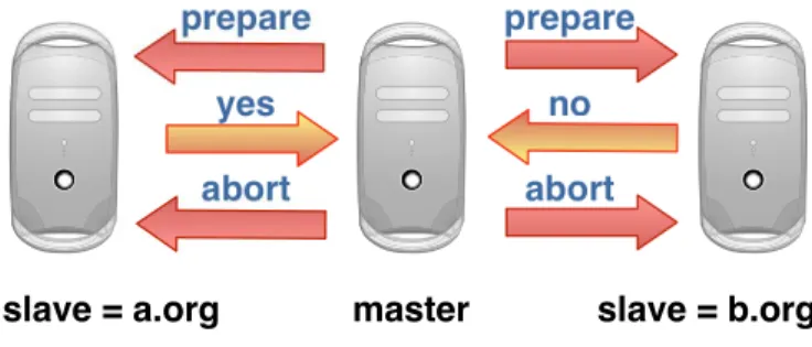
master
slave = a.org slave = b.org
prepare prepare
no yes
abort abort
Figure 2.3: An example of simulation running on Neko’s real network mode
Chapter 3
Simulator Model
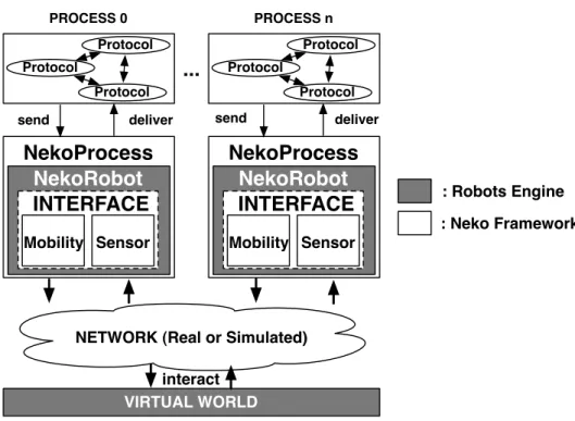
In this chapter, we are going to talk about the specification of simulator model. The figure 3.1 shows overall model after we have integrated mobile robot engine with the original Neko’s model. As for robots engine, we have 2 layers which are interface layer and virtual world layer.The interface layer provides control for robots mobility and sensor modules to user.Virtual world layer is the layer of simulated world that robots are existing in. As a result, the integration of mobility and communication can be ensured. We can let robot move in virtual world while having them send/receive messages using Neko.
VIRTUAL WORLD interact Protocol
Protocol
Protocol
Protocol
Protocol
Protocol
PROCESS 0 PROCESS n
...
NekoProcess
deliver deliver
send send
NETWORK (Real or Simulated)
NekoProcess
NekoRobot
Mobility
INTERFACE
Sensor
NekoProcess NekoRobot
Mobility
INTERFACE
Sensor
: Robots Engine : Neko Framework
Figure 3.1: Overall Model after integrated robots engine with Neko
Next we will explain about each components in this model. The simulator’s model can be divided as the following sections,
3.1 Mobile Robots
Mobile robots are the objects those have the capability to move around in their environ- ment and are not fixed to one physical location as industrial robots, which usually are attached to a fixed surface.
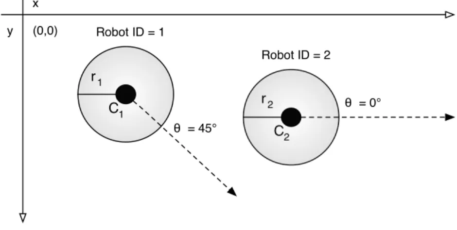
In this simulator, robots are designed based on the real physical robots model. To say specifically, each mobile robot is represented as a the process that logically has its own memory, processing unit and control separately from other robots. In software level, robots contain the following programmatic data informations. For an example of robot definition please refer to figure 3.2.
(0,0) y
x
Robot ID = 2
= 0°
r2 C2 Robot ID = 1
= 45°
r1 C1
Figure 3.2: Robot id 1 facing to 45 degree and robot id 2 facing to 0 degree
• ID Number
A unique identity number of each robot in the simulation system.
• Size
Size (or to say volume) of the robot, represent by using radius value. Currently this simulator supports only the circular-shaped robot which has same length in both width and height.
• Angle
Angle, is the degree of angle that robot is facing to at a certain time. The angle will be calculated from the origin point (0,0) count anti-clockwise to the target angle.
3.1.1 Motion Modules
Firstly, the most important thing for the mobile robot system is their motions. Robots motions are represented with vector movement. In this simulator, we describe a robots motion as a vector from the their depart coordination to their destination. See figure 3.4 for more understanding.
Robot 1
Robot 2
wheel-based motion module
leg-based motion module
turn
forward
backward
move digonal move straight
move side
..
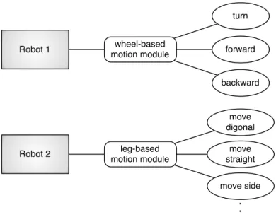
Figure 3.3: An example of varies motion modules.
Motion module is the module that let robot move in the virtual environment. The motion module is also can be called actuator in physical robot. It it is the module that will tell how a robot move. A robot may attached difference motion modules from the others and using totally difference motion patterns. For instance, a wheel-based robot and a spider-shape robot might be attached with difference motion module and move dif- ferently. Furthermore, depending on developer,a robot might be attached with multiple motion modules and provides varies motion pattern.
Each motion module consists of one motion pattern or many motion patterns that they are providing. For instance, a wheel-based robot’s motion module may provide a turn,
= 90°
r1 C1 (0,0)
y x
r1 NewC1 F(t) = VectorNC1
Figure 3.4: A motion vector that was generated by the motion module.
R1
x y (0,0)
R1 R1
X(t start)
X(t)
X(t finish)
: motion vector at a certain time : motion path
Figure 3.5: An example of motion vector calculation.
forward and backward motion pattern. See figure 3.3 for an instance of motion module.
A motion pattern’s main task is vector calculating and generating. To put it simply, it get a motion request from robot, then calculate the vector of motion from that request.
Therefore, any motion pattern that can be calculated with the mathematic equation can be created as a motion pattern. Developers are allowed to create their own motion pat- tern for robots as long as that motion pattern can be described in equation and return the correct motion vector for the robot at a certain time. See figure 3.5 for the vector calculation mechanism in each motion pattern.
Currently, our simulator provides a basic motion module which designed based on the movement of wheel-based robot. A basic motion module (or to say a default motion module) contains three motion patterns, which should sufficient for testing distributed
robots algorithm that concentrate on the interaction between robots or groups of them.
However, as previously said, developers are also having the option to develop their own motion pattern in the case that the evaluation of complex motion is necessary. As long as the developers follow the philosophy of the framework, the extended motion patterns can be seamlessly integrated to the this simulator easily.
The calculation of default motion module that was integrated to this simulator can be derived into the following equation,
N ewCoordination =DepartCoordination+−−−−−→V elocity∗t (3.1) Alternatively, we can rewrite this equation into the following short notation term.
X(t) =X(0)+V ∗t (3.2)
X(t) refers to robot’s position at the time t while X(0) represents the position of its position before start moving and V is the speed vector that contains direction.
As for the default motion module, it provides these following motion patterns,
• TURN
A motion pattern that let robot turn around itself by using its center point as a turning pin point. The calculation for this motion pattern is nothing than a addition of angles. The motion vector produced by this motion pattern is a unit vector that contains only direction (because when turning robot stay in the same place).
• FORWARD
A motion pattern that allow robot to move to the direction that it is facing to.
Since the robot just moving straight with this motion pattern, the angle will be the same as depart angle.
• MOVETO
A motion pattern that combine a turn and a forward motion pattern together. It works with global positioning system by calculating angle that it needed to turn to the destination coordination, then do the turn motion pattern to that target angle,then after the turning is finished, it move forward to the destination coordi- nation.
3.1.2 Sensors
Sensor is a module that let robot ask information of itself, other robots or environment from the system. Robots are separately running from the others. They have no any shared memory or shared processing unit. Therefore it has to request the information of surrounding environment via its sensors. In this simulator we divided sensors into two groups as the following.
• Pull-model based sensors (a.k.a. Query-based sensors)
ROBOT 1
SENSOR MANAGER
" I want to know my coordination "
" OK. Here is your coordination "
Figure 3.6: An example of pull-model based sensor.
These sensors are the query-based sensors. They will receive a sensor request from robot at a certain time, then wait for the reply from the system and forward that reply after it came to robot. These sensors are called pull-model based sensors.
Examples of sensors in this category are gps sensor and view sensor.
• Push-model based sensors (a.k.a. Notification-based sensors)
SENSOR MANAGER
ROBOT 2 ROBOT
1
" Someone's in your view ! "
V
Figure 3.7: An example of push-model based sensor.
These sensors are opposite with above query-based sensors. They will automatically repeat the sensoring mechanism with the time-interval for each sensoring period.
They works asynchronously with robots after they have been activated. While they
are re-sensoring with a interval period, if the interrupt condition has become true they will send an interrupt message to robots and give them a sensor’s reply message.
These sensors are called push-model based sensors. An example of a sensor in the category is a proximity sensor. Proximity sensor will interrupt and send a sensor message to robot if there is other robot try to get into the sensor range (aka. sensor’s view size) of this robot.
3.2 Virtual Environment
Virtual environment (also know as virtual world)is the virtual plane-area that is simulated based on the real-world model’s space. It is a space that robots are existing and moving in. All of the actions from robots are happening in this simulated world. In this simulator, virtual world based on the Cartesian coordinate system which composed of the x-axis and y-axis. The virtual world might be limited for the size in x-axis and y-axis, or might be an infinity space.
3.3 Collision
Collision is the event that a robot collide with another object and lead to the collision’s effect between those objects. Actually in mobile robots system, collision can be cate- gorized into two groups, which are collision between robots and collision between robot and obstacles. However, currently our simulator support only the detection of collision between robots.
This collision happen by the one or more robots moving near to the other until the distance between their’s border is become zero, that made robots borders are touching together (also known as collision). We also can separate the collision between robots into two subgroups, which are the collision between moving robots, and the collision between a moving robot and a idling robot. As for the second case, when a robot is not moving and is in idle state, it will become an obstacle for the other robots those are moving in the system.
The other collision that our simulator does not support but should be mentioned is the collision between robot and obstacle. This group of collision is the collision that occur between a robot and an obstacle object in virtual world. As previously said, the virtual world might not be only a simply plane space. It might be a space that consists of many
obstacle objects in its area. The obstacle might be a object that is simulated from the real-world’s objects such as a rock, a car or even a wall. Whatever that are, they all do the same role, that is, blocking a moving robot from going further.
In fact, considering real-world model, obstacle object may be very vary and not limited to just the objects those blocking robots way. For instance, a river may not block a robot from moving but just slow its movement down (in the case that robot failure from wetting is not considered). Or another example, a hole that robot can fall into and partly damage, or even completely fall and disappear from the system. However, our simulator’s aim is to making the framework as simple as it can in order to reduce the complexity in user’s setting. Hence, currently our simulator does not provide support for such a complex ob- stacle yet.
3.4 Robot’s Communications
After we have talked about robots components and their virtual world, in this section we are going to talk about their communication.
As previously described in chapter 2, Neko’s original purpose is for rapid prototyping distributed algorithm. In order to simulate the environment for those distributed algo- rithms, network management ability has a very important role for this field of simulations.
In order to support those simulations, Neko provide the ability to allow user to experiment their algorithm on both real network and simulated network. Neko also concentrates on the reusability and encapsulation of communication’s protocols which this feature can be considered as Neko’s strongest point.
After we have successfully developed the mobility model on the top layer of Neko, we moved to the next phase and integrated it with Neko’s communication framework. As a result our simulator now support both robots mobility and their message transmissions.
Now we go back to mobile robot’s world. In the cooperative mobile robots simulation, in some models the motioning and sensoring might not enough for evaluating an algorithm because we are not simulating just one robot. We are talking about multiple groups of robots which each group might consists of a very big amount of robots like one thousand
or ten thousand robots. In order to effectively controls those robots and increase the throughput for this robot system, the cooperation between them is an extremely crucial factor.
We have known that the cooperation between them is very importance, but how can they cooperate to each others? There are two methods that they can provides cooper- ation to each others. First is by using a sensor. A robot might use a sensor to check the situation around them and if necessary it may provide help for other robots. For an instance, a leader robot uses a view sensor to check number of robots in a certain area. If some robots are falling behind it will wait for them. If all robots have already gathered in the destined area, a leader robot will start moving and lead the group to the next target. Other than using sensor, the second method is by using communication which is the main purpose of this section. Since each robots are having their own processing unit and memory, they do not have a shared memory so that they can share information together. In order to share a certain information to other robots, a robot has to do the transmission (aka. communication).
robot 1
robot 3
robot 2
send() at T 0
receive() at T 1
receive() at T 2
INTERFACE NETWORK
NEKO's NETWORK
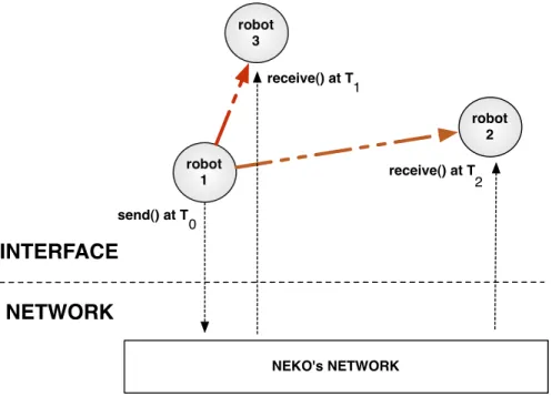
Figure 3.8: An example of a robot broadcasting a message to other two robots In this simulator, Neko’s network framework has been used for simulating communica- tion environment. As we see in the figure 3.8, in the interface layer we can see a robot
broadcasted a message to other robots at time T0. However, in the back-end mechanism the robot did not send a message to other robots directly. It sent a message to Neko’s sim- ulated network (as seen in figure 3.8 as network layer). Then the simulated network will generate delay of message and order of receivers based on the communication algorithms (aka. microprotocols, will be explained in the next section) that have been using. After that, the message will be successfully delivered to the target robots eventually, which is the delivering of messages at T1 and T2 in the example in figure 3.8.
3.5 Microprotocol Framework
In this section, we are going to talk about the philosophy of a framework called micropro- tocol framework. The Neko distributed algorithm prototyping toolkit that we extended the mobility model for, was entirely based on the microprotocol framework’s philosophy.
Or to say it concretely, Neko was firstly developed on the traditional protocol stacks and was re-factored to completely support microprotocol framework later.
Before getting in to the detail of microprotocol framework, we would like to briefly talk about the traditional protocol stacks. Protocol stacks have been used as a set of collaborating components which these components are called layers. The arrangement of layer’s order and communication patterns are fixed, which made each layer can only com- municate with the layers directly above and below itself. In order to solve this limitation and provides more flexibility and reusability in framework, the newer framework with new philosophy has been proposed. The framework is called microprotocol framework.
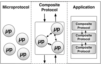
Microprotocol framework, is the framework that permitting the use of finer grained components called microprotocols. Microprotocols are small structuring units that are self-contained and clear in what service that are providing. The basic promise of micro- protocol framework is a full separation of concerns between programming microprotocols and composing them. Therefore these two tasks can be carried out by different people with a minimal interaction. This feature can be called multi-level programming. For more understanding see figure 3.9.
From the figure 3.9, the finer grained structuring unit (left side) is called microproto- cols. The people who define the definition and develop these microprotocols are called
μp
Microprotocol Composite
Protocol Application
Composite Protocol Composite
Protocol Composite
Protocol
μp μp μp
μp μp
μp
Figure 3.9: Multi-level programing support in microprotocol framework microprotocols programmers.
Next, the components in the middle part of this figure is called composite protocols.
Depends on the author the name calling this type of components might difference. Other developers sometime calls them as complex microprotocols or protocol layers.
Composite protocol is the set of multiple microprotocols and their interconnections.
Developers in this programming level are called microprotocols composers. Microprotocol composers are able to plug microprotocols together, without having to know or change the code of the microprotocols.
Last, the final part on the right side is an application. The application consists of mul- tiple composite protocols that are working together while linking by the interconnections between them. Though normally developer in this programming level is usually the same team with microprotocol composer, however in a complex application the application pro- grammers may be assigned to this programming level separating from composers.
In figure 3.10 we created an example of distributed algorithm for communication using microprotocol’s philosophy. This application consists of 4 microprotcols that are providing their own services, which are the following units.
• Atomic Broadcast
This protocol module implements atomic broadcast (aka. Total-order broadcast).
NETWORK Process 1 (Robot 1)
...
Atomic Broadcast
μP
Consensus μP
Failure Detection
μP Leader Election
μP
Process n (Robot n)
Atomic Broadcast
μP
Consensus μP
Failure Detection
μP Leader Election
μP
Figure 3.10: An example of application using microprotocol’s philosophy
The mechanism is to deliver a message to all receiver nodes same order with sending order. It interacts with consensus module both for solving consensus and failure detection purpose.
• Consensus
This protocol module implements an algorithm for solving consensus problem. It interacts with failure detection module to monitor and detect an unreliable node.
It also interacts with leader election in case that the new leader is needed.
• Leader Election
This protocol module suggests a new leader to application. It interacts with con- sensus to ensure same agreement for all nodes.
• Failure detection
This protocol module implements a failure detection based on network condition.
For ex., using ping messages. It interacts with consensus for permitting the same agreement on suspected node.
In previous example of microprotocol-based application, with the advantage of micro-
protocol framework, the composer does not needed to know the programming code in each microprotocols. The composer can easily create a complex application by just plugging microprotocols together without having to change the code in microprotocols.
Now we have talked both mobility model for mobile robots system and communication framework on Neko. As a result, the combination of mobility model and microprotocols- based communication framework of Neko make it possible for developers to create a prototype of complex application of cooperative mobile robots system. We believe that this approach will lead us to more effective way for rapid prototyping cooperative mobile robots application which has the needs for evaluating on both mobility and communica- tions algorithms.
3.6 Discrete Event Simulation Engine
The engine of this simulator is implemented based on the discrete event simulation en- gine. Discrete event simulation is a simulation system that represented as a chronological sequence of events. Each event occurs at an instant time and make a change of state to the system. Since each event happen in an instance time, the mechanism do not pay attention to the interval between events. Only the event at a certain time will be recorded and marked to the system. Some other reference report also called the time-management system for discrete event simulation engine as time-warp mechanism.
Originally the discrete event simulation’s philosophy was suitable for the system that the change of state can be marked to the system as a new event. However, as for mobile robots system, when we want to implement the discrete event simulation system to robots simulation engine, there were several difficulties in implementation which will be spoken in the following part.
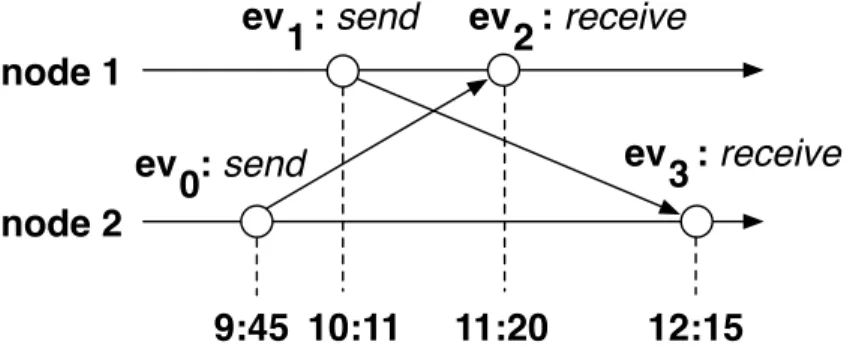
Unlike physical-time system that use the sequence time system like the real world’s time (see fig.3.11), the discrete event simulation engine’s time-warp mechanism cannot provide the information of system’s state in the interval period between two events (see fig.3.12). For the system like network simulation system, there might be no problem with marking only message in/out events. But, considering robot system, marking only their depart and arrive event is the same meaning with robot are doing the teleportation (aka.
warping).
node 1
node 2
ev2
ev0
ev1
ev3
9:45 10:11 11:20 12:15 : send
: send : receive
: receive
Figure 3.11: An example of physical time system.
at 9:45 ev 0 : send
ev1 ev3 ev
2
ORDER: ev0 ev1 ev2 ev3
event queue
Figure 3.12: An example of virtual time system in discrete event simulation In mobile robot system, each robot is alway moving on the coordination in virtual space. That means their positions (or to say states in the system) are always changing.
Therefore, in some situation the information from the marked depart event and arrive event might be inadequate. For an example, a robot depart from point A at 7th second and will arrive at point B at 10th second. However, what if we want to let the sensor check the position of this robot at 8th second? Since the system only marked the depart and arrive event, how can we know the exact position of this robot at 8th second? See the figure of this example situation at fig.3.13
As for the solution, we can get the information on that interval-period between two events by using vector calculation. As previously said, a robot’s motion can be repre- sented as a vector of movement. All vectors of movement in this simulation system can
ROBOT 1 S A VIRTUAL
TIME
0 .. 7 8 9 10 ..
S : Start Moving Event : Sensor Event A : Arriving Event
Figure 3.13: A figure shows robot requesting sensor while it is moving
be derived with the equation from equation 3.2 which is X(t) =X(0)+V ∗t. While X(t) refers to robot’s position at the time t and X(0) represents the position of its position before start moving and V is the speed vector that contains direction. As a result, with the above equation we can get exact coordination of a robot at any time t and be able to solve the previous positioning query problem.
However, on the good side, in spite of the lacking of state’s information in the interval period between two events, marking robot’s motion as a depart and arrive event will dra- matically increase the speed of simulation. For example, if we implement the simulation of a group of robots with physical-time based simulator. In the case that robot’s speed is extremely slow or the distance to move is very far, the simulation might take a very long time to finish all robots actions. But, with the discrete event simulation engine’s virtual time system, the system will jump to the arrive events of all robots in an instant time.
As a result, with the discrete simulation engine’s mechanism the simulation time can be incredibly shortened.
Chapter 4
Simulator Architecture
The content in this chapter is about the system architecture implemented in this simulator.
The explanation starts from overall big-picture of the simulator system then concretely detailed about each component and then an explanation about output from simulation.
4.1 Overall Architecture
The structure consists of three layers. Algorithm layer, interface layer and engine layer.
Algorithm layer is the top-level layer which each robot’s algorithm is defined and imple- mented in this layer. To put it simply, in this layer developers only concern about the moving algorithm for each robot. Next layer is the interface layer, the layer that play the role of interface between developer and robot’s programmatic codes. Last is the bottom layer, the engine layer. This layer represents back-end core engine of the simulator. All requests received from interface layer are handled here and then processed into simulation output. For more understanding refer to figure 4.1.
The simulator composed of the following core components,
• Motion Modules
The modules that allow robots to move.
• Sensors
The modules that help robots ask information from the system.
• Managers
The modules in the back-end engine that entirely manage their own field of tasks.
SENSOR ACTUATOR SENSOR
ACTUATOR SENSORSENSOR SENSORSENSOR
Motion Command
Motion/Sensor Request Motion/Sensor
Request
Motion Command Sensor
Command
Sensor Event Motion /
Collision Event
Motion Manager
Collision Detector Sensor Command
Sensor Manager
Algorithm 1 Algorithm 2
Robot n
ACTUATOR SENSOR
Virtual World Robot 1
ACTUATOR SENSOR
Queued Event
Event Manager Sensor
Reply
Sensor Reply
...
...
Algorithm Layer
Interface Layer
Engine
Layer infomation
request
infomation request
Figure 4.1: Overall structure of simulation system
• Virtual World
The virtual space simulating logical world for all robots.
In the next section we are going to explain these components in the detail.
4.2 Components
4.2.1 Motion Modules
Motion module is a component that allow a robot to move in the virtual world. Since the basic model of this module has already been talked in chapter 3, in this section we are going to explain about the programmatic mechanism.
As been said previously, the simulator is based on the discrete event simulation’s phi- losophy. That means all of the actions from robots will be translated in to records of changes in system’s state at a certain time, which these records will be called events.
For robots motions, we translate their motion requests to motion events by using mo- tion manager, then register these events into event queue. When a motion request is translated to motion events, normally two events will be produced. These events are start event and finish event. However, some complex motions may required to produce more than traditional start event and end event. For an instance, a MOVETO motion request (moving robot to the target destination) may requires start-turning event, finish-turning event, start-forwarding event and finish-forwarding event.
Considering more complex motion patterns those might be extended to the simulator in the future, we provide an interface for the motion module which requires user to define two operations (aka. methods in JAVA). The first operation is the calculation part of the motion module, which required to be able to provide the coordination of a robot at any time t. With the event-based simulation system, events will instantly happen at certain time. However, robots are always moving and resulting in the change of their global coordinations. Hence a method to calculate robots position at any target time is necessary for each motion. The returned value is a MotionVector datatype, which is a vector of motion of that robot at time t. Second operation is the returning of array of motion events occur from the motion. As previously said, a complex motion may produces multiple events other than start and finish event, considering extendability, the declaration of this operation is unavoidable. See reference figure at fig.4.2.
calMotionVector() getMotionEvent()
<<Interface>>
MotionInterface
calMotionVector() getMotionEvents() motionName
TurnMotion
calMotionVector() getMotionEvents() motionName
Forward Motion
Figure 4.2: Motion modules in UML diagram
TURN Motion
A motion that turn a robot with a target degree in angle. Related calculations are the following,
N ewAngle= (P reviousAngle+−−−−−−−−−→T urnV elocity∗t)%2π (4.1) N ewCoordination=DepartCoordination (4.2) Events happened from this motion : Start-turn and finish-turn event.
FORWARD Motion
A motion that make robot moving forward in to the direction that it is facing to with a certain distance. Related calculations are as the following,
N ewAngle=P reviousAngle (4.3)
N ewCoordination =DepartCoordination+−−−−−→V elocity∗t (4.4)
−−−−−→
V elocityX−axis =M oveSpeed∗cos(angle) (4.5)
−−−−−→
V elocityY−axis =M oveSpeed∗sin(angle) (4.6) Events happened from this motion: Start-forward and finish-forward event.
MOVETO Motion
A motion that combined tun motion and forward motion together. Make robot move to a destination point by calculating the degree needed to turn and distance to move, then do the turning and forwarding sequentially.
Events happened from this motion:
Start-turn, finish-turn, start-forward and finish-forward event.
4.2.2 Sensors
The next components that we are going to talk in this section are sensors. Sensor is a module that robots use for asking information from the system (or environment). A robot usually equipped with more than one sensor module. In programmatic software level, a mobile robot may be represented as the collection of multiple sensors which are integrated into a moving object. Without sensors, a robot can not know the information of the outside world.
doSensor() calReply()
AbstractSensor
doSensor() calReply() sensorName
GPS Sensor
doSensor() calReply() sensorName
View Sensor
activate() inactivate() setTimeInterval()
<<Interface>>
Push Sensor
activate() inactivate() setTimeInterval() calReply() sensorName timeInterval
Proximity Sensor
Figure 4.3: Sensor modules in UML diagram In this simulator we divided sensors into two groups as following.
Pull Model’s Sensor
Sensors in this group is called push-model’s sensors. They will work using a query-based mechanism, which is sending a sensor request to system and then wait for the reply to return back to the requester robot.
As for the mechanism of pull-sensoring operation in this simulator, first a robot uses its sensor and request for an information of the system. For instance, a position request or surrounding view request. After that, the request will be sent to sensor manager and transform into a sensor event waiting for the time to be triggered. After the sensor event has been triggered, the requested sensor will use informations of the system it get pro- vided by sensor manager, then calculate the result for this request and then return a reply to requester robot as a SensorReply datatype. Since the reply answer’s datatype may be difference depending on the sensor’s type. For instance, gps sensor might return a Point2D position of requester robot but view sensor will return an array of positions of robots in view range. Hence, the message containing in SensorReply will be stored as a instance of Object class in java. It will be correctly casted into the right datatype before return the reply to the requester robot.
Each sensor will be extended from the provided sensor abstract class. A sensor is needed to define two operations which are doSensor() method and calReply() method. A doSensor() method is the main interface method providing to the robot (or to say to the
user). A robot will ask for a sensor request using this method, then a sensor reply will eventually returned to the robot. Due to the vary types of sensors, parameters required by this method are difference. For instance, a gps sensor may not require any parameter for sensoring operation, but a view sensor requires the range of view in order to perform sensoring operation. Next operation that is needed to be declared is named calReply() method. This method is the back-end calculation part of each sensor. After a sensor event is triggered, this method will be called in order to calculate the reply for a certain request at a event’s trigger time. See figure 4.3 for more understanding.
The following sensors are the pull model-based sensors those are provided in the simu- lator as default modules.
• GPS sensor
A sensor that provide robot’s global coordination at request time.
• View sensor
A sensor that return an array of position of robots those are in the range of sensor’s view size.
• Proximity sensor
A sensor that return an array of distance to objects in the range of sensor’s view size.
Note that the proximity sensor can be both pull model-based and push model-based sensor.
Push Model’s Sensor
Sensors in this group are called push model’s sensors. They are sensors that waiting for an activation, and after they have been activated they will automatically do the sensoring operation with a time interval until they get inactivated or the simulation is finished.
The push model-based sensor will not always return the sensor reply to a robot every time they do sensoring, but they will return the sensor reply to a robot only when the interrupt condition has become true. For instance, though a proximity sensor was set to re-sensoring in every 5 second of time interval, it will interrupt a robot and return the sensor reply only when there is a robot come closer into the sensor’s view range in order to warn the robot before the collision happen.
Except the re-activating with a time interval mechanism, the main sensoring operation is similar to previously spoken pull model-based sensors. Therefore the push model-based
sensors extends an abstract sensor class as pull model-based sensors do. However, in or- der to support for the re-activation mechanism, they are required to implements another interface called PushSensorInterface. See figure 4.3 for more understanding.
Below are the push model-based sensors those are provided in the simulator as default modules.
• Proximity sensor
A sensor that will send an interrupting sensor reply to warn a robot if there is another robot come closer into sensor’s view range.
• Contact sensor
A sensor that will warn a robot if a robot has touched with other robots or objects.
4.2.3 Managers
After we have known the motion and sensor modules, in this section we are going to explain about the manager classes. These manager hander the requests from robot and manage the system in the back-end. They also provide the collection of many useful meth- ods for the other modules in their management area. Because of the data encapsulation, only the manager-class’s components have authority to access to virtual world’s informa- tions. The other modules are allowed only to request those information via their manager.
The manager classes in this simulator are as the following.
Motion Manager
Motion manager is the core component that handle entire motion operations for all robots.
Motion manager provides many of useful functions those related to robot mobility. It also responsible for the collision detection for the robots. The task of motion manager starts right after there is a motion request sent from robot. It will update the system’s state (aka. all robots statuses) to current time before doing any calculation. Then it will analyze the motion request that received from requester robot and transform into motion events. At this point, motion manager have known that there was a change to the system.
Therefore it will detect for the collision which may happen from the new motion request.
If there will be any collision occur, it will create the collision event and ask event manager to register both the new motion events and the collision event to event queue. If there
was no any collision found it will just register only the new motion events. See figure 4.4 for reference.
Receive MotionRequest
Update Statuses
Detect Collision
isThereCollision?
START
Register Collision Events
Initial Motion Events
Register Motion Events
FINISH
no
yes
Figure 4.4: Flow chart of the motion manager’s working mechanism for one motion request
Sensor Manager
Sensor manager controls most of the main operations relating to sensor system. It starts the work after the sensor request was sent from a robot. Before do any calculation, it update the system’s state to current time same way with motion manager do. Then it will create the sensor event from the sensor request it received from the robot and then ask event manager to register this sensor event to event queue. In the same time, it checks whether this sensor request is a push sensor request or pull sensor request. If this request was a request from pull sensor, it will register the new sensor event and the task will finish here. However in the case of push sensor request, an optional task of re-activating sensor is needed. Therefore, if this request is a push sensor request, after the new sensor event has been registered, it will wait for the time interval of the requester push sensor and then repeat the sensor operation again at the next time interval. It will repeat this
mechanism until that push sensor is inactivated or the simulation has finished. See figure 4.5 for reference.
Receive sensor request
Create sensor event
Register sensor event
isPushSensor? START
Wait for Time Interval
yes
no FINISH
sensor event is triggered
Return sensor reply to requester robot
Interrupt condition =
true?
Interrupt robot and return sensor reply
no
yes
Figure 4.5: Flow chart of the sensor manager’s working mechanism
Event Manager
Event manager is the manager that controls all of the task related to events in the system.
It has an event queue that stores all of the events of the system. All of the operations related to event management has to be done by the event manager only. The main services that it is providing are event registering and event canceling/removing. It also provides a function to return an array of events stored in the queue for any target robot in the case that developer want to check the future-events of a robot before performing an extra action.
4.2.4 Virtual World
Virtual world is a logical space that robots are existing in. It is a almighty module that knows everything about the robots without having to be told from the other modules. It
is the heart of the simulation engine which storing all of the robots statuses at the current simulation time. The state of each robots will be updated from time to time (specifically say, every time a new event is triggered). The virtual world ensures that the statuses of all robots storing in itself will always up-to-date with the current simulation time. A direct access from an external module to virtual world’s database is strictly prohibited due to the data encapsulation. Only the manager-class’s components have the authority to access its database.
4.3 Events
All of the state changing (aka. check point) in the system are represented as events.
Every time an event is triggered, something happens and mark the change of state to the system. Except for the sensor event that will just ask the information from the system and then return that data to the requester robot. In this section, we are going to explain about the detail of each event.
However, before that we have to know that there are two types of event in this simulator which are eventually-happen event and conditional event.
• Eventually-Happen Event
Events in this group are the traditional event that eventually-happen in the system.
The events will be marked with the trigger time. Whatever happen, as long as the simulation has not been terminated, they will certain happen at their trigger time.
The events in this group are, motion-start event and sensor event.
• Conditional Event
Events in this group are as its name, in some condition they might not happen in the system and get removed from the event queue. For an instance, a collision event that has been registered to system at t0 and should happen at t3, will be canceled if the robot change its motion path before t3. Because it has changed its path before the collision take place. In contrast, if the collision event happened, the motion-finish event will be canceled instead. In conclusion, events in this groups are motion-finish event and collision event.
4.3.1 Motion Event
A motion event represents the change of a robot’s position and its status. It will be marked to the system whenever it get triggered. Below is the flowchart show operations
related to motion events since the time event is created until it finished its task and is removed from the event queue. A motion request from robot will be processed into a motion-start event and a motion-finish event.
Motion Event is created and
registered
Wait until trigger time
Motion Event is triggered START
FINISH Motion Event is removed
Virtual World is updated
Figure 4.6: Flow chart of the operations related to motion events
4.3.2 Sensor Event
A sensor event is like a request of a snapshot of the system. It will not mark any new state to the system like motion event do, but it will do a snapshot of the system, get information from the system at a certain time, then process this information, transform the information into sensor reply and return to requester robot. Below is the flowchart show operations related to sensor events since the time event is created until it finished its task and is removed from the event queue.
Sensor Event is created and
registered
Wait until trigger time
Sensor Event is triggered START
FINISH Sensor Event is removed
Sensor Reply is generated and returned to robot
Figure 4.7: Flow chart of the operations related to sensor events
4.3.3 Collision Event
Collision event is a difference from motion event and sensor event. Because collision event is a conditional event. To put it simply, even a collision event has already been registered into the system, depending on the condition of the robot, this collision event might not
happen and get canceled. The condition that make a collision event get canceled is the changing in motion of a robot after the collision event was registered. For instance, robot A and robot B are moving. With current direction and velocity, the collision between them was detected at t0 and should happen at the time t2. However, at the time t1 (which t1 happen before t2) robot B has changed it movement and go to a difference coordination.
At this point, the previous collision will become invalid and has to be canceled. The motion manager has to do the collision detection again in time t1. Below is the flowchart show operations related to collision events since the time event is created until it finished its task and is removed from the event queue.
no yes
Collision Event is created and
registered
Wait until trigger time
Collision Event is triggered START
FINISH
Virtual World is updated
is there new motion request
before trigger time?
Collision Event is canceled Collision Event
is removed
All Future Events of this robot are canceled and removed
Figure 4.8: Flow chart of the operations related to collision events
4.4 Collision Detection
In this section we are going to explain about the collision detection mechanism using in this simulator. Collision detection operation has a very importance role in motion robot simulation. Because many of robots algorithms have the ultimately goal to effective utilize their limited resource. Therefore, if a collision occurred in system that means we are losing our resource in some ways (robots, energy or even a time). Because of that reason, we aware of the important of the collision detection in the robot simulation system and have integrated this mechanism into our simulator’s engine.
Before get into the detail of the mechanism used in our simulator, we would like to talk about the popular mechanism being used for collision detecting. We divided the methods that frequently used for detecting collision in robots simulation into two groups
as following.
• Detecting using time slice
This type of detection mechanism has been using in a number of mobile robot sim- ulators including Player/Stage[2]. It works by slicing the time period that a robot do moving action into many smaller time intervals. Then repeatedly detect for the collision at every time interval. To put it simply, it is the mechanism that put many checkpoints into the system to observe each robot’s movement. For instance, a robot requests to do a movement action which will start at 1stsecondand finish in 10thsecond. The collision detector knows that this motion will consume 10seconds to finish. However, it does not know where and when the collision will occur. There- fore it slices that 10seconds period in to many smaller time intervals. Let’s assume that it sliced with the time interval of 2second. Hence, the collision will be checked at 3rdsecond, 5thsecond, 7thsecond and 9thsecond.
tstart t
finish
1 10
: Motion Event
Figure 4.9: Before doing the time slicing
tstart t
finish
1 2 3 4 5 6 7 8 9 10
: Checkpoint for collision detection
Figure 4.10: After the time slicing have done
This method has both advantages and trade-offs. The good side is, the mechanism itself is easy to implement because the detector does not have to consider about the future-events. It just let the system run and perform the detection at every checkpoints. Furthermore, while using this method we do not have to worry about the shape of robots. They can be any shape because the detector does not have to
predict any collision by using geometrical calculation. It just let the system run and take a checkpoint at every interval.
However, there are several trade-offs in this method as well. First, the number of steps in calculating is incredibly big. Because it needs to calculate at every time- interval, hence the steps number of calculation has became as following,
N umberOf Steps =T imeU sage÷IntervalBetweenChecking (4.7) The other drawback for this method is the accuracy in detecting. The bigger time interval between each checkpoint the less accuracy in detecting. For instance, let’s use the above example that a robot want to do a movement action from 1stsecond to 10thsecond. Let’s assume that a collision should happen in 8thsecondif the robot does not change its course. With the time-slice method, if the time interval is equal or less than 1second, it should be able to successfully detect a collision at 8thsecond.
However, in the case that interval period is bigger than 1second, the collision might not be found. Let’s demonstrate with 3seconds interval period. In this case the detector will do the checking at 4thsecond, 7thsecond and 10thsecond. As a result, no collision was found. Or it might be found but later than the time that it should happen which is 8thsecond. Using extremely small interval period may solve this problem in some case, however the steps number of calculation will incredibly in- creased and the efficiency of the simulator will dramatically drop.
With above drawbacks of this method, we decided to implements out simulator’s collision detector with other method which will be explained in the following part.
• Detecting using mathematic equation
This detection method is the method that uses mathematic calculation. The detec- tor will use current statuses of all robots for detecting the collision that will happen in the future. We knows that a robot’s motion can be represented as a motion vector at a certain time. More precisely say, their motion vector at a certain time can be calculated from the equation X(t) = X(0)+V ∗t while X(t) is the position of th robot at timet. Therefore, the detector will use this equation to calculate the collision that will occur in the future. From now we are going to talk about how can it detect for the collision using mathematic equations.