Direct computation of knot Floer homology and the Upsilon invariant

(1)

Direct computation of knot Floer homology and the Upsilon invariant

Taketo Sano (The University of Tokyo)^∗

Abstract

By using grid homology theory, we give an explicit algorithm for computing Ozsv´ath-Stipsicz-Szab´o’s Υ-invariant and thed-invariant of Dehn surgeries along knots in S³. As an application, we have computed these invariants for all prime knots with crossing number up to 11¹. This is a joint work with Kouki Sato.

1. Introduction

The Υ-invariant defined by Ozsv´ath, Stipsicz and Szab´o [7] is a group homomorphism Υ : C →PL([0,2],R),

whereC denotes the smooth knot concordance group and PL([0,2],R) the vector space of piecewise-linear functions on [0,2]. The d-invariant defined by Ozsv´ath and Szab´o [5] is a group homomorphism

d: θ^c →Q,

where θ^c denotes the Spin^c rational homology cobordism group of Spin^c rational homology 3-spheres (see [5, Definition 1.1] for the precise definition ofθ^c). Here we focus on the d-invariant ofS_p/q³ (K), the rational p/q-surgery along a knot K inS³.

These invariants were originally defined in different packages of Heegaard Floer theory, but later Livingston [1] and Ni-Wu [4] have translated them into the words of the doubly filtered chain complex CF K^∞ defined in [6]. Manolescu, Ozsv´ath and Sarkar introduced a combinatorial description of CF K^∞, which is called the grid homology theory. The difficulty in computing algorithmically the above mentioned invariants is thatCF K^∞involves heavy analitic machinery, while the grid complex is combinatorial but is generated over a multivariate Laurent polynomial ringF[U₁^±1,· · · , U_n^±1].

We have overcome this difficulty by considering Sato’sG0-invariant [9] in the context of grid homology theory. G₀ is originally defined using CF K^∞, and both invariants Υ_K andd(S_p/q³ (K)) can be obtained from it. We have translated this invariant into the context of grid homology theory, and developed an explicit algorithm for computing it. As an application, we have computed Υ_K and d(S_p/q³ (K)) for all prime knots with crossing number up to 11. A more detailed paper is to be submitted to arXiv soon.

2. Preliminary

2.1. The G₀-invariant

A subset R∈Z² is called a closed region if

(i, j)∈R, (k, l)≤(i, j) ⇒ (k, l)∈R.

In other words, a closed region is alower set with respect to the partial order≤ ofZ². Given a knotK ⊂S³, we denoteC =CF K^∞(K), which is aZ²-filtered chain complex

∗e-mail:[email protected]

1At the time of the talk, there were 5 remaining knots whose Υ-invariants haven’t been computed

(2)

generated over F[U, U⁻¹]. A closed region R gives a subcomplex C_R of C, where each element ofC_R is a sum of elements xsuch that the two gradings (Alex(x),Alg(x)) lies inR. The set of all closed regions of Z² gives aZ²-filtration onC.

It is known that H₀(C)∼=F for any knot K. Ge₀(K) is defined as a set of all closed regionsR such thatC_R contains a homological generator ofH₀(C). This is equivalent to saying that the natural map H₀(C_R)→H₀(C) is surjective. The invariant G₀(K) is defined as the minimal subset ofGe0(K) with respect to the partial order ⊂ of P(Z²).

Theorem 2.1 ([9, Thereom 5.1]). Both Ge₀(K) and G₀(K) are knot concordance invariants. (More strongly, they are invariant under ν⁺-equivalence.)

Theorem 2.2 ([9, Theorem 5.7]). G0(K) is non-empty and finite.

In the following we explain that the invariants Υ_K andd(S_p/q³ (K)) can be obtained fromG₀(K). First we explain the translation of {d(S_p/q³ (K))}p/q∈Q>0 intoNi-Wu’s V_k- sequence{V_k(K)}k∈Z≥0 [4]. Note that there is a canonical identification between the set of Spin^c structures over S_p/q³ (K) and {i|0≤i≤p−1} (see [8, Section 4, Section 7]).

Let d(S_p/q³ (K), i) denote the correction term of S_p/q³ (K) with the i-th Spin^c structure (0≤i≤p−1).

Proposition 2.3 ([4, Proposition 1.6]). For coprime integers p, q >0, the equality d(S_p/q³ (K), i) =d(S_p/q³ (O), i)−2 maxn

V_bⁱ

qc(K), V_b^p+q−1−i

q c(K)o

holds, where O denotes the unknot and b·c is the floor function.

Theorem 2.4 ([9, Proposition 5.17]). For a knot K, the invariants Υ_K(t) and V_k(K) are determined from G₀(K) by the formulas:

V_k(K) = min{m∈Z≥0 | ∃R∈ G₀(K), R⊂R_(m,k+m)} Υ_K(t) =−2 min{s∈R| ∃R∈ G₀(K), R⊂R^t(s)}

where the regions R_(k,l) and R^t(s) are defined as:

R_(k,l) :={(i, j)∈Z² |i≤k and j ≤l}, R^t(s) :=

(i, j)∈Z²

(1− t 2)i+ t

2j ≤s

.

2.2. Grid homology theory

First we review the construction of a grid complex. Agrid diagram G lies on ann×n grid of squares (the numbern is called the grid number of G), where some squares are decorated either with an O or an X so that

• every row contains exactly oneO and one X;

• every column contains exactly one O and one X.

Given such data, one obtains a planar link diagram by drawing horizontal segments from theO’s to the X’s in each row, and vertical segments from the X’s to the O’s in each column, while letting the horizontal segment underpass the vertical segment at every intersection point (see Figure 1). It is known that every link inS³ possesses such representation. We usually place the diagram in the standard plane so that bottom left corner is at the origin, each square has length one, and each O and each X is centered

(3)

Figure 1: Grid diagram and the corresponding knot

at a half-integer point. We set O={O_i}_1≤i≤n, X={X_i}_1≤i≤n so that eachO_i and X_i has its center inx=i− ¹₂.

Given a grid diagram G, the chain complex C⁻(G) is constructed as follows. First we regardGas a diagram on the torus by gluing the two opposite sides. The generating set S is given by n-tuples of intersection points between the horizontal and vertical circles, with the property that each horizontal (or vertical) circle contains exactly one intersection point. Eachx∈S can be identified with the set of permutations of length n under the correspondence

σ 7→x={(i, σ(i))}0≤i<n.

C⁻(G) is generated by S over the multivariate polynomial ringF[U₁,· · · , U_n]. The differential ∂ is defined as

∂(x) =X

y∈S

X

r∈Rect^◦(x,y)

U₁¹· · ·U_nⁿy

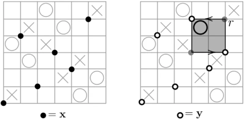
where Rect^◦(x,y) denotes the set of empty rectangles connecting x to y (which exist only whenxandy are related by a single transposition), and for each empty rectangle r, the exponenti ∈ {0,1}is given by the number of intersections ofrandOi. Figure 2 depicts an empty rectangle r connecting xto y, and for thisr we have ₄ = 1. See [3]

for the precise definition.

=x =y

r

Figure 2: An empty rectangle connecting x toy

C⁻(G) is endowed the Maslov grading and the Alexander grading. Each x ∈ S is assigned two integers M(x), A(x) ∈ Z. Also each factor U_i is declared to decrease M by −2 and A by −1. Then it is proved that ∂ decreases M by −1, while A is non-increasing under ∂. Thus M gives a homological grading of C⁻(G), while A gives a filtration on C⁻(G).

(4)

Theorem 2.5 ([2, Theorem 3.3]). C⁻(G) is filtered chain homotopy equivalent to CF K⁻(K).

There is another filtration defined on C⁻(G), that is the algebraic filtration. For any element of the form U₁^a¹· · ·U_N^a^Nx∈C⁻(G), we define

Alg(U₁^a¹· · ·U_N^a^Nx) =−a₁.

With these two filtrations,C⁻(G) becomes aZ²-filtered chain complex. As in the case of CF K^∞, for any closed region R⊂Z², this is a corresponding subcomplex C⁻(G)_R.

3. Translating G₀ into grid homology theory

For any closed region R, we define itsshift number by

shift(R) := max{i∈Z| ∃j ∈Z s.t. (i, j)∈R}.

Also for any integer s≥0, we define the shifted region:

R[s] := {(i, j)∈Z² |(i+s, j+s)∈R}.

Obviously whens = shift(R),

shift(R[s]) = 0 holds.

Theorem 3.1. Let K be a knot with grid diagram G. Denote C = C⁻(G). Let R be a closed region with shift(R) = s. Then R ∈ Ge0(K) if and only if C_R[s] contains a homological generator of degree −2s.

4. The algorithm

In the following we assume that we are given a grid diagram G = (O,X) of K as an input.

4.1. Enumerating the candidate regions

For each coordinate (k, l)∈Z², the simple region R_(k,l) is defined as R_(k,l):={(i, j)∈Z² |i≤k and j ≤l}.

The following two propositions are consequences of [9].

Proposition 4.1. For any g ≥0,

G₀(T_2,2g+1) = {R(i,g−i) |i= 0,· · · , g},

G₀((T_2,2g+1)^∗) = {R(−g,0)∪R(−g+1,−1)∪ · · · ∪R(0,−g)}

Proposition 4.2. Let g₃, g₄ denote the 3-, 4- genus of the knot K respectively. Any R∈ G₀(K) satisfies the following conditions:

1. Each corner (i, j) of R satisfies |i−j| ≤g₃.

2. R includes the region R_(−g₄_,0)∪R_(−g₄_+1,−1)∪ · · · ∪R_(0,−g₄₎.

3. If R contains a point (i, g₄−i) for some i∈ {0, . . . , g₄}, then R =R_(i,g₄−i). Thus any corner (i, j) ofR ∈ G₀(K) lies in the bounded area,

|i+j| ≤g₄ (ij ≥0),

|i−j| ≤g₃ (ij <0).

hence we obtain a finite set of candidate regions.

(5)

4.2. Enumerating the generators

Recall the generating setSof the grid complexC⁻(G) corresponds one-to-one with the set of permutations of length n. C⁻(G) is generated by S over the ringF[U₁,· · · , U_n], which is not suitable for computation. We inflate the generators by multiplying mono- mials and regard C⁻(G) as an (infinitely generated) chain complex over F. Since each factor U_i decreases the homological degree by 2, for any k ∈ Z, the k-th chain group C_k⁻(G) can be regarded as a finite dimensional vector space over F with generators of the form

U₁^a¹· · ·U_N^a^Nx, degx−2P

ia_i =k.

We call generators of this form inflated generators. Obviously the number of inflated generators increases combinatorially as the homological degree k decreases.

4.3. Computing the homological generator of degree 0

Next the algorithm computes a homological generator of degree 0, i.e. a representative cycle of the unique generator of H₀⁻(G)∼=F. Since each chain group is a finite dimensional vector space over F, it is possible to compute the cycle directly. In practice we use a more effective method, but we here omit the details.

4.4. Determining the realizability

Having prepared one homological generator z of degree 0, we are ready to determine the realizability of the candidate regions. For any s ≥ 0, the element (U₁)^sz gives a homological generator of degree −2s. From Theorem 3.1, a closed region R of shift number s is realizable if and only if there is a cycle homologous to (U₁)^sz that is contained in C_R[s]. This is equivalent to the condition that (the image of) (U₁)^sz is null homologous in the quotient complex Q_R := C/C_R[s]. For any k ∈ Z, we can take a finite basis of (Q_R)_k from the inflated generators contained in C_k and modding out those contained in (C_R[s])_k. Having fixed such bases in degree −2s and −2s+ 1, the differential ∂ : (Q_R)−2s+1 → (Q_R)−2s is represented by a matrix A. Thus the realizability of R is equivalent to the existence of a solutionx of the linear system

Ax=b

where b is the vector corresponding to (U₁)^sz ∈ (Q_R)−2s. Now that we have reduced the problem to linear systems, the remaining task is purely computational.

Now, in theory,G₀is algorithmically computable by checking the realizability for all candidate regions. However, such computation would be extremely expensive even for a relatively small grid diagram. We have developed many more reduction techniques that would make computations feasible for prime knots of crossing number up to 11.

References

[1] Charles Livingston. Notes on the knot concordance invariant upsilon. Algebr. Geom.

Topol., 17(1):111–130, 2017.

[2] Ciprian Manolescu, Peter Ozsv´ath, and Sucharit Sarkar. A combinatorial description of knot Floer homology. Ann. of Math. (2), 169(2):633–660, 2009.

[3] Ciprian Manolescu, Peter Ozsváth, Zoltán Szabó, and Dylan Thurston. On combinatorial link Floer homology. Geom. Topol., 11:2339–2412, 2007.

[4] Yi Ni and Zhongtao Wu. Cosmetic surgeries on knots in S³. J. Reine Angew. Math., 706:1–17, 2015.

(6)

[5] Peter Ozsváth and Zoltán Szabó. Absolutely graded Floer homologies and intersection forms for four-manifolds with boundary. Adv. Math., 173(2):179–261, 2003.

[6] Peter Ozsváth and Zoltán Szabó. Holomorphic disks and knot invariants. Adv. Math., 186(1):58–116, 2004.

[7] Peter S. Ozsváth, András I. Stipsicz, and Zoltán Szabó. Concordance homomorphisms from knot Floer homology. Adv. Math., 315:366–426, 2017.

[8] Peter S. Ozsváth and Zoltán Szabó. Knot Floer homology and rational surgeries. Algebr.

Geom. Topol., 11(1):1–68, 2011.

[9] Kouki Sato. The ν⁺-equivalence classes of genus one knots. arXiv e-prints, page arXiv:1907.09116, Jul 2019.