Geochemical study for dissolved methane in the high latitude ocean〜the Sea of Okhotsk and the Southern Ocean〜

(1)

Table of Contents

Chapter 1 General Introduction 1.1 How much is the global warming?

1.2 Global methane budget 1.3 Methane in the ocean 1.4 Objectives of this study

Chapter 2 Methane in the western part of the Sea of Okhotsk in boreal summer 1998‑2000

2.1 Introduction

2.2 Materials and Methods 2.3 Results and Discussion

2.3.1 Methane distribution east of Sakhalin 2.3.2 Methane distributions in the northwestern

continental shelf zone

2.3.3 Methane flux between sea and air in the western Sea of Okhotsk

2.3.4 Vertical and lateral transport of methane off east Sakhalin

2.4 Summary

Chapter 3 Methane in the South Pacific and Southern Ocean in austral summer 2001‑2002

3.1 Introduction

3.2 Materials and Methods 3.3 Results and Discussion

3.3.1 Methane in the South Pacific 3.3.2 Methane in the Southern Ocean 3.3.3 Summary

Chapter 4 Global estimates of oceanic methane and General outlook

4.1 Global estimates of oceanic methane 4.2 Methane in the high latitude ocean 4.3 Comparison with sea-air flux

4.4 General Outlook Acknowledgments References

Chapter 1 General Introduction

1.1 How much is the global warming?

The estimate of global surface temperature change is a 0.6℃ increase since the late 19th century with a 95% confidence interval of 0.4 to 0.8℃. The increase in temperature of 0.15 ℃ compared to that assessed in the IPCC WGI Second Assessment Report ［IPCC,1996］is partly due to the additional data for the last five years, together with improved methods of analysis and the fact that the SAR decided not to update the value in the First Assessment Report, despite slight additional warming. It is likely that there have been real differences between the rate of warming in the troposphere and the surface over the last twenty years, which are not fully under- stood. New palaeoclimate analyses for the last 1,000 years over the Northern Hemisphere indicate that the magnitude of 20th century warming is likely to have been the largest of any century during this period. In addition, the 1990s are likely to have been the warmest decade of the millennium. New analyses indicate that the global ocean has warmed significantly since the late 1940s:more than half of the increase in heat content has occurred in the upper 300 m, mainly since the late 1950s. The warming is superimposed on strong global decadal variability.

Night minimum temperatures are continuing to increase, lengthening the freeze-free season in many mid-and high latitude regions. There has

Laboratory of Environmental Geochemistry, Department of Biosphere and Environmental Sciences, Faculty of Environ- ment Systems, Rakuno Gakuen University, Ebetsu, Hokkaido, 069‑8501, Japan

本稿は，北海道大学大学院地球環境科学研究科審査博士論文である。

Geochemical study for dissolved methane in the high latitude ocean

〜 the Sea of Okhotsk and the Southern Ocean 〜

Osamu Y

OSHIDA (Accepted 13 January 2009)

(2)

been a reduction in the frequency of extreme low temperatures, without an equivalent increase in the frequency of extreme high temperatures.

Over the last twenty-five years, it is likely that atmospheric water vapor has increased over the Northern Hemisphere in many regions. There has been quite a widespread reduction in daily and other sub-monthly time-scales of temperature variability during the 20th century. New evidence shows a decline in Arctic sea-ice extent, particularly in spring and summer. Consistent with this finding are analyses showing a near 40%

decrease in the average thickness of summer Arctic sea ice over approximately the last thirty years, though uncertainties are difficult to estimate and the influence of multi-decadal variability cannot yet be assessed. Widespread increases are likely to have occurred in the pro- portion of total precipitation derived from heavy and extreme precipitation events over land in the mid-and high latitudes of the Northern Hemi- sphere.

1.2 Global methane budget

Methane(CH )is an atmospheric trace gas that contributes about 20% to the greenhouse effect,it is the second most in importance as a greenhouse gas after CO . Atmospheric levels of methane have varied by a factor of 2 and such variations have paralleled variation in global mean temperature over the same period.

Methaneʼs globally averaged atmospheric surface abundance in 1998 was 1,745 ppb,corresponding to a total burden of about 4,850 Tg CH . The uncertainty in the burden is small ( ±5%)because the spatial and temporal distributions of tropospheric and stratospheric CH have been determined by extensive high-precision measurements and the tropospheric variability is relatively small. For example, the Northern Hemisphere CH abundances average about 5% higher than those in the Southern Hemisphere. Seasonal variations, with a minimum in late summer, are observed with peak-to-peak amplitudes of about 2% at mid-latitudes. The average vertical gradient in the troposphere is negligible, but CH abundances in the stratosphere decrease rapidly

with altitude, e.g., to 1,400 ppb at 30 km altitude in the tropics and to 500 ppb at 30 km in high latitude northern winter.

The most important known sources of atmospheric methane are listed in IPCC ［2001］. Although the major source terms of atmospheric methane have probably been identified, many of the source strengths are still uncertain due to the difficulty in assessing the global emission rates of the biospheric sources,whose strengths are highly variable in space and time: e.g., local emissions from most types of natural wetland can vary by a few orders of magnitude over a few meters.

Nevertheless, new approaches have led to improved estimates of the global emissions rates from some source types. For instance,intensive studies on emissions from rice agriculture have substantially improved these emissions estimates

［Ding and Wang, 1996;Wang and Shangguan, 1996］. Further, integration of emissions over a whole growth period (rather than looking at the emissions on individual days with different ambient temperatures) has lowered the estimates of CH emissions from rice agriculture from about 80 Tg y to about 40 Tg y ［Neue and Sass, 1998;Sass et al., 1999］. There have also been attempts to deduce emission rates from observed spatial and temporal distributions of atmospheric methane through inverse modeling ［e.g.,Hein et al.,1997;Houweling et al. ,1999］. The emissions so derived depend on the precise knowledge of the mean global loss rate and represent a relative attribution into aggregated sources of similar properties. The results of some of these studies have been included in IPCC［2001 ］. The global methane budget can also be constrained by measurements of stable isotopes (δ C and δD) and radiocarbon ( CH )in atmospheric methane and in CH from the major sources ［e.g.,Stevens and Engelkemeir, 1988;Wahlen et al. , 1989;Quay et al., 1991, 1999;Lassey et al. , 1993;Lowe et al., 1994］. So far the measurements of isotopic com- position of CH have served mainly to constrain the contribution from fossil fuel related sources.

The emissions from the various sources sum up to a global total of about 600 Tg y ,of which about 60% are related to human activities such as

Osamu Y

(3)

agriculture, fossil fuel use and waste disposal.

This is consistent with the SRES estimate of 347 Tg y for anthropogenic CH emissions in the year 2000.

The current emissions from CH hydrate deposits appear small, about 10 Tg y . How- ever,these deposits are enormous,about 107 Tg C

［Suess et al.,1999］,and there is an indication of a catastrophic release of a gaseous carbon com- pound about 55 million years ago,which has been attributed to a large-scale perturbation of CH hydrate deposits［Dickens,1999;Norris and Rohl, 1999］. Recent research points to regional releases of CH from clathrates in ocean sediments during the last 60,000 years［Kennett et al., 2000］, but much of this CH is likely to be oxid- ized by bacteria before reaching the atmosphere

［Dickens, 2001］. This evidence adds to the con- cern that the expected global warming may lead to an increase in these emissions and thus to another positive feedback in the climate system.

So far, the size of that feedback has not been quantified. On the other hand, the historic record of atmospheric methane derived from ice cores［Petit et al., 1999］ , which spans several large temperature swings plus glaciations, con- strains the possible past releases from methane hydrates to the atmosphere. Indeed,Brook et al.

［2000］find little evidence for rapid,massive CH excursions that might be associated with large- scale decomposition of methane hydrates in sediments during the past 50,000 years.

The mean global loss rate of atmospheric methane is dominated by its reaction with OH in the troposphere.

OH＋CH → CH ＋H O

This loss term can be quantified with relatively good accuracy based on the mean global OH concentration derived from the methyl chloroform (CH CCl )budget described on OH. In that way we obtain a mean global loss rate of 507 Tg CH y for the current tropospheric removal of CH by OH. In addition there are other minor removal processes for atmospheric CH . Reac- tion with Cl atoms in the marine boundary layer probably constitutes less than 2% of the total sink

［Singh et al., 1996］. A recent process model

study［Ridgwell et al.,1999］suggested a soil sink of 38 Tg y , and this can be compared to SAR estimates of 30 Tg y . Minor amounts of CH are also destroyed in the stratosphere by reac- tions with OH, Cl, and O(1D), resulting in a com- bined loss rate of 40 Tg y . Summing these,the best estimate of the current global loss rate of atmospheric methane totals 576 Tg y , which agrees reasonably with the total sources derived from process models. The atmospheric lifetime of CH derived from this loss rate and the global burden is 8.4 years. Attributing individual life- times to the different components of CH loss results in 9.6 years for loss due to tropospheric OH, 120 years for stratospheric loss, and 160 years for the soil sink (i.e., 1/8.4y＝ 1/9.6y＋ 1/120y＋ 1/160y).

The atmospheric abundance of CH has increased by about a factor of 2.5 since the pre- industrial era as evidenced by measurements of CH in air extracted from ice cores and firn

［Etheridge et al., 1998］. This increase still con- tinues, albeit at a declining rate. The global tropospheric methane growth rate averaged over the period 1992 through 1998 is about 4.9 ppb y , corresponding to an average annual increase in atmospheric burden of 14 Tg. Superimposed on this long-term decline in growth rate are interan- nual variations in the trend. There are no clear quantitative explanations for this variability,but understanding these variations in trend will ulti- mately help constrain specific budget terms.

After the eruption of Mt.Pinatubo, a large positive anomaly in growth rate was observed at tropical latitudes. It has been attributed to short-term decreases in solar UV in the tropics immediately following the eruption that decreased OH formation rates in the troposphere

［Dlugokencky et al., 1996］. A large decrease in growth was observed, particularly in high northern latitudes, in 1992. This feature has been attributed in part to decreased northern wetland emission rates resulting from anomalously low surface temperatures［Hogan and Harriss, 1994 ］ and in part to stratospheric ozone depletion that increased tropospheric OH［Bekki et al. , 1994;

Fuglestvedt et al., 1994］. Records of changes in

(4)

the C/C ratios in atmospheric CH during this period suggest the existence of an anomaly in the sources or sinks involving more than one causal factor［Lowe et al., 1997;Mak et al. , 2000］.

There is no consensus on the causes of the long-term decline in the annual growth rate.

Assuming a constant mean atmospheric lifetime of CH of 8.9 years as derived by Prinn et al.

［1995］,Dlugokencky et al.［1998］suggest that during the period 1984 to 1997 global emissions were essentially constant and that the decline in annual growth rate was caused by an approach to steady state between global emissions and atmospheric loss rate. Their estimated average source strength was about 550 Tg y .(Inclusion of a soil sink term of 30 Tg y would decrease the lifetime to 8.6 years and suggest an average source strength of about 570 Tg y .) Francey et al.［1999］, using measurements of CH from Antarctic firn air samples and archived air from Cape Grim, Tasmania, also concluded that the decreased CH growth rate was consistent with constant OH and constant or very slowly increasing CH sources after 1982. However, other analyses of the global methyl chloroform (CH CCl )budget［Krol et al.,1998］and the changing chemistry of the atmosphere［Karlsdottir and Isaksen, 2000］argue for an increase in globally averaged OH of＋0.5% y over the last two decades and hence a parallel increase in global CH emissions by＋0.5% y .

The historic record of atmospheric CH obtained from ice cores has been extended to 420,000 years before present ［Petit et al., 1999］. CH varies with climate as does CO . High values are observed during interglacial periods, but these maxima barely exceed the immediate pre-industrial CH mixing ratio of 700 ppb. At the same time, ice core measurements from Greenland and Antarctica indicate that during the Holocene CH had a pole-to-pole difference of about 44±7 ppb with higher values in the Arctic as today, but long before humans influenced atmospheric methane concentrations ［Chappelaz et al., 1997］. Finally, study of CH ice-core records at high time resolution reveals no evidence for rapid, massive CH excursions that

might be associated with large-scale decomposition of methane hydrates in sediments［Brook et al., 2000］.

1.3 Methane in the ocean

The oceans are believed to represent a source for atmospheric methane. This conclusion is based on the observation that the surface water of the ocean is usually supersaturated with respect to atmospheric methane. Supersaturation with methane has been observed at most stations in the world oceans. In order to understand the current global methane cycle, it is necessary to quantify its sources. At present,there remain large uncertainties in the estimated methane fluxes from sources to sinks. The oceanʼ s source strength for atmospheric methane should be examined in more detail,even though it might be a relatively minor source, reported to be 0.005% to 3% of the total input to the atmosphere［Conrad and Seiler,1988;

Cicerone and Oremland,1988;Bange et al.,1994］. Historically, the methane flux from the ocean has been estimated mainly from measurements of methane concentration in the surface water of the open oceans［Ehhalt, 1974 ］. In the open oceans, the surface water is slightly supersaturated with atmospheric methane. On the other hand, remarkable supersaturation in coastal regions, including continental shelf zones,has been reported. Owens et al.［1991］measured methane in the Arabian Sea and reported larger emission rate to the atmosphere (0.04 Tg y ), as compared with previous studies. Bange et al. ［1994］ re- evaluated the methane data in previous studies and reported that the degree of supersaturation was 200‑500% in the Black Sea,95 ‑12,000% in the southern North Sea, and 120 ‑23,900% in the northwestern Gulf of Mexico. Watanabe et al.

［1994］showed that the flux of methane(3.8×10 mol CH km d )in Funka Bay,Japan,was 2 to 3 orders of magnitude larger than values estimated in the open oceans［e.g.,Cicerone and Oremland, 1988］. Tsurushima et al.［1996 ］reported that the flux of methane in the East China Sea was somewhat larger than oceanic values.

Most of the known marine methane hydrate res- ervoirs are located along the continental margins

Osamu Y

(5)

［Gornitz and Fung, 1994］. Rehder et al.［2000］ reported that the enhancement of CH fluxes to the atmosphere in regions of coastal upwelling is likely to occur on global scale. Although coastal seas occupy about1/10 of the open ocean area

［Bange et al.,1994］,the degree of supersaturation there is about 1 order of magnitude greater than that in the open oceans. However,methane data from coastal regions are too scarce to allow the global methane flux to be estimated precisely.

Several reports showed that the vertical profile of methane concentration has the maximum at subsurface layer in the Ocean but the origin of its maximum is not clear. Suggestion includes advection from nearby sources in shelf sediments, diffusion and/or advection from local anoxic environments, and in situ production by methanogenic bacteria,presumably in association with suspended particulate material. Some observations suggested that biogenic methane production occurred in the subsurface layer. In the water column,although only the methanogenic bacteria produce methane, they cannot survive under any traces of oxygen. Therefore, these bacteria are thought to probably live in the anaerobic microenvironments supplied by organic particles or guts of zooplankton［e.g., Alldredge and Cohen, 1987］. Recently,it is reported that some amount of methane is released by zooplankton- phytoplankton co-culture in the laboratory. But, there was few data that prove environmental subsurface methane production. In the Southern Ocean, large size zooplanktons such as Antarctic Krill and Sulpa live in great numbers, so in this area,much of methane seems to be formed in guts of zooplankton.

1.4 Objectives of this study

This study focused specially and temporally in detail profile of methane concentration and distribution in the water column. Fig.1 shows the observation area taken up in this paper.

The Sea of Okhotsk taken up in chapter 2 has focused on the behavior of the oceanic biogenic methane in the coastal zone, the thermogenic methane off Sakhalin,and the effect of the Amur River water inflow. In addition in this chapter,it

is indicated to be available taking the anomalously high methane concentration as a chemical tracer.

The South Pacific Ocean taken up in chapter 3 indicates that it focuses on the behavior of the methane in the open ocean, and that the concentration of methane in the open ocean increases gently in comparison with past and present surface water saturation.

The Southern Ocean taken up in the same chapter 3 has focused on the biogenic methane formed in the organic particle and guts of zooplankton. In this area, there is a good correlation of methane concentration with chlorophyll a concentration;it seems to be formed by Antarctic zooplankton.

While much of methane seemed to have been formed in these high latitude Oceans characterized by the high biological productivity in summer and the active vertical mixing in winter, the methane in the ocean hardly was observed. The estimates how much is the methane discharged to the atmosphere from these oceans are uncertainty. By clarifying spatial features of the marine methane supply to the atmosphere,it is a purpose of this study to reduce the uncertainty as a source of the ocean for atmospheric methane.

Characteristics in each area are described at each following chapters.

Fig.1.Observation station taken up in this paper (XP98, XP99, XP2000, KH‑01‑3, JARE 43 Tangaroa cruise).

(6)

Chapter 2 Methane in the western part of the Sea of Okhotsk in boreal summer 1998‑2000

2.1 Introduction

The Sea of Okhotsk is one of the largest marginal seas, and is the important location for the ventilation of the North Pacific Intermediate Water characterized by a salinity minimum centered at 26.8 σ. Therefore in recent years oceanographic studies have been made extensive- ly［Ohshima et al., 2002;Mizuta et al., 2003］. Lammers et al.［1995］measured methane in the surface waters off the northeast coast of Sakhalin (52°30ʼ‑53°30ʼN, 143°20ʼ‑144°30ʼE) in the western part of the Sea of Okhotsk. They reported seasonal variations in the methane flux between the sea and the air due to methane concentrations ranging from 385 nM under the ice in winter to 6 nM in the ice-free midsummer. The magnitude of supersaturation indicates that the Sea of Ok- hotsk is a significant source of atmospheric methane. Ginsburg et al.［1993 ］reported gas hydrates and gas-vent fields in the Sea of Okhotsk on the northeastern continental slope off Sakhalin (53.2‑54.6°N, 144.0‑144.7°E), and Cranston et al.

［1994］found methane hydrates of thermogenic origin there. Natural gas is extracted from the large oil and gas fields there (e.g., http: //src- home.slav.hokudai.ac.jp/sakhalin/eng/71/akaha.

html). Despite extensive seepage of thermogenic methane from sediments, there are only a few reports of the temporal and spatial variations in methane flux to the atmosphere and the processes controlling it.

As part of the Joint Japanese―Russian―U.S.

Study of the Sea of Okhotsk,we measured methane concentrations throughout the water column in the western part of the Sea of Okhotsk during the three cruises in July ‑August 1998, August‑ September 1999, and June‑July 2000 (Fig.2).

Here we report the distribution of methane released from sedimentary and thermogenic sources, and estimate the flux of methane from the western part of the Sea of Okhotsk to the atmosphere.

2.2 Materials and Methods

During the three cruises, we collected about 1700 seawater samples at hydrographic stations (dots in Fig.2),using the R/V Professor Khromov of the Far Eastern Regional Hydrometeorological Research Institute,Russia. In July ‑August 1998, the surface seawater samples were collected in a 1-L bucket, and other samples were collected from 5‑25 depths from the surface (2 m) to the bottom in 10‑L Niskin bottles. Each sample was carefully subsampled into a 30 ‑mL glass vial so as to avoid contamination by air. The seawater samples were poisoned with 0.5 mL of mercuric chloride solution［Tilbrook and Karl, 1995;

Watanabe et al., 1995］, and then the vials were closed with rubber and aluminum caps. They were stored in a cool, dark place until the gas chromatographic analysis of methane in our laboratory on land.

The analytical method was similar to that of

Fig.2.Water sampling locations during the cruises of July‑August 1998, August ‑September 1999, and June‑July 2000. The dotted line shows the area where we estimated the methane flux between the sea and the air (see Table 2).The capital letters A to H indicate survey transects and the numbers 1 to 4 indicate the station for discussion (see Figure 15). NE means the area of northeastern Sakhalin shelf,NW means the area of the northwestern continental shelf,and CE means the central region of the Sea of Okhotsk.

Osamu Y

(7)

Tsurushima et al.［1996］, briefly described here.

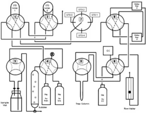
The system consists of a purge and trap unit, a desiccant unit, rotary valves, a gas chromatograph (Shimadzu GC‑8A) equipped with a flame ionization detector, and a data acquisition unit (Fig.3). The whole volume of seawater in each 30‑mL glass vial was processed all at once to avoid contamination and loss of methane ［Yo- shida et al., 2004］.

The precision obtained from replicate determi- nations of methane concentration was estimated to be better than 5% for the usual concentration of methane in seawater. The standard gases used contained 2.48 ppmv (Takachiho Chemical Industrial Co.Ltd)and 38.4 ppmv (Nippon Sanso Co.Ltd)of methane in pure nitrogen.

2.3 Results and Discussion

2.3.1 Methane distribution east of Sakhalin East of Sakhalin, the methane concentrations showed prominent features in waters close to the

bottom and between the subsurface and surface mixed layers.

2.3.1.1 Thermogenic methane in waters over the northeastern shelf

In waters over the northeastern shelf, anomalously high concentrations of methane were observed near the bottom (Figs.4 ‑6) of the eastern shelfbreak at a depth of 〜200 m, due to methane seepage from an underlying oil field

［Ginsburg et al., 1993;Lammers et al., 1995］. Maximum emission rate of methane from sediments was estimated based on maximum concentration of methane and flow rate of seawater (Table 1). The highest concentration of methane existed in water with a density of 26.6 ‑26.8 σ (corresponding to the Okhotsk Sea Intermediate Water), a relatively low temperature, a low nitrate concentration, and a high dissolved oxygen concentration every year (Fig.7). The anomalously high concentrations of methane oc-

Fig.3.Flow diagram of the gas chromatograph analysis.

Table 1.Maximum CH emission rate from sediments (mg CH m d )

Section year

1998 1999 2000

B 1.8 4.1 2.3

C 2.0 0.8 1.7

D 0.3 0.2 0.3

(8)

curred among the dense shelf water, which is probably originated from the northwestern shelf area and transported by the East Sakhalin Cur- rent［e.g.,Kitani,1973;Talley,1991;Yamamoto et al., 2002］.

The methane concentration in the near-bottom water along section E was relatively low compared with those of sections B and C to the south, showing clearly that the thermogenic methane sources are not uniformly distributed geographi- cally along the shelf northeast of Sakhalin. The highest methane concentration in sections B and C varied temporally and spatially:488 nmol kg in July‑August 1998 (section C), 981 nmol kg in August‑September 1999 (section B),and 556 nmol kg in June‑July 2000 (section B). There are two possible sources of changes in methane con- Fig.4.Distribution of methane concentrations along

section B in (a)July‑August 1998, (b)August ‑ September 1999, and (c) June‑July 2000. The dotted lines show water with a density of 26.6 ‑ 26.8 σ.

Fig.5.As for Figure 4 except in section C.

Fig.6.Distribution of methane concentrations along section E in (a)August‑ September 1999,and (b) June‑July 2000. The dotted lines show water with a density of 26.6‑ 26.8 σ.

Osamu Y

(9)

centration:variations in methane flux from thermogenic sources and lateral transport by the East Sakhalin Current.

The highest methane along section C, east of 145.5°E, was found in subsurface water with a density of 26.6‑26.8 σ in 1998 and 1999,but not in 2000 (Fig.5). In open oceans, the highest methane concentration is commonly found in the subsurface water［e.g.,Ward et al.,1987;Conrad and Seiler,1988］,as explained by a decrease in biological methane production with depth［Karl and Tilbrook, 1994］and a high rate of loss from the surface layer［Jayakumar et al. , 2001］. Along section C,the subsurface maximum concentration of methane was too high to explain by in situ production via biological activities. In the northeastern Sea of Okhotsk, extremely high concen-

trations of methane caused by major thermogenic methane sources have also been reported ［Lam- mers et al.,1995,based on Geodekyan et al.,1976］. The subsurface maximum east of 145.5°E may have been caused by the southwestward transport of thermogenic methane from northeastern latitudes［Ohshima et al., 2002］.

Along section D (Fig.8), at stations close to Sakhalin (west of 146°E), the maximum methane concentration (61 nmol kg ) occurred in water with a density of 27σ in July ‑August 1998. This result also indicates relatively large thermogenic methane emission for the year. As found in the area northeast of Sakhalin, these methane concentrations varied significantly from year to year:

43 nmol kg in August‑September 1999,80 nmol

Fig.7.(a)Distribution of methane,(b)temperature,(c) nitrate concentration,and (d)dissolved oxygen concentration along section B in June ‑July 2000. The dotted lines show water with a density of 26.6‑26.8 σ.

Fig.8.Distribution of methane concentrations along section D in July‑August 1998, August‑

September 1999, and June‑July 2000. The dotted lines show water with a density of 26.6‑26.8 σ.

(10)

kg in June‑July 2000.

2.3.1.2 Methane distribution in surface sea water

-

Surface seawater over the shelf northeast of Sakhalin, the methane concentration had ranged from 3 to 42 nmol kg in July ‑August 1998,from 3 to 14 nmol kg in August ‑September 1999,and from 4 to 80 nmol kg in June ‑July 2000 (Fig.9).

In a layer of 50‑200 m depth of the western part, its concentration showed a steep gradient between the subsurface and surface mixed layers, while in the eastern part remained fairly constant.

In the eastern part of sections B and C and the northern part of section A, the methane concentrations in the surface mixed layer (〜20 m) ranged from 3 to 5 nmol kg ,approximately equal to or slightly larger values reported in the open oceans (Figs.7, 8, and 10).

Along the eastern Sakhalin coast,the existence

of less-saline surface seawater originating from the Amur River has been reported ［Itoh and Ohshima, 2000］. From the vertical profiles of temperature and salinity, a strong stratification in the upper〜10 m (an example is shown in Fig.

11) was observed. We surmise that the strong stratification due to freshwater inputs from the Amur River restricted the underlying methane- rich water from ventilating. For example,along section C, freshwater input from the Amur River was observed in August‑ September 1999, but not clearly in June‑July 2000.

Consequently, the surface methane concentration was relatively low in 1999,while high in 2000, although the 1999 maximum methane concentration in the near-bottom water was larger than that in 2000 (Fig.12).

Relatively high concentrations of methane were observed at almost all the stations with the shall- owest depth (＜〜100 m) near the coast. From the observations of near-surface circulation and tidal currents in the Sea of Okhotsk, Ohshima et al.［2002］have found amplification of the diurnal tidal current near the coastal region east of Sakhalin. Their observational results suggest that the high methane concentration in the sur-

Fig.9.Longitudinal distributions of methane in surface seawater and bottom depth along (a)section E,(b)section B,and (c)section C over the shelf northeast of Sakhalin.

Fig.10.Distribution of methane concentrations in water with a density of 26.8σ in July ‑August 1998.

Osamu Y

(11)

face water observed near the coastal region may be caused by the active tidal mixing there. As another possibility for the high methane concentration of the coastal surface water, a wind- driven mixing effect should be relatively small, because of weak wind in summer.

2.3.1.3 Vertical profile of methane concentra tions in the central region

-

The anomalously high methane concentrations along sections B and C can be used to trace the water with a density of 26.6 ‑26.8 σ in the East Sakhalin Current. Methane distribution in such water in 1998 showed higher concentrations ( ＞7 nmol kg ) over the shelf east of Sakhalin (Fig.

10). In the central region north of 50°N, the methane concentration east of the shelfbreak

decreased considerably to the level of 3 nmol kg , while south of 50°N relatively high concentration (〜5 nmol kg ) was observed. This distribution of methane was mainly controlled by the transport of methane from the source region in the shelf northeast of Sakhalin. The East Sak- halin Current can be divided into two parts,southward flow along the coast and southeastward flow away from the coast of Sakhalin ［Ohshima et al., 2002］;our results also support its current pattern.

2.3.2 Methane distributions in the northwest ern continental shelf zone

-

2.3.2.1 Methane north of Sakhalin

North to northwest of Sakhalin (section F),the methane concentration in the near-bottom water

Fig.11.Vertical profiles of(a)methane concentration,(b)emperature,and (c)salinity in the upper 30 m over the shelf northeast of Sakhalin (54°N, 143.8°E).

Fig.12.Distributions of methane and salinity in surface water along section C in August‑September 1999 and June‑ July 2000.

(12)

was higher than that in the surface water and fairly constant over a wide area north of 54.5° N (Fig.13). The methane is thought to be discharged by microorganisms in the sediments into the water column［Ward et al. , 1987;Conrad and Seiler,1988;Kvenvolden et al. ,1993;Bange et al., 1994, 1998;Tsurushima et al., 1996;Jayakumar et al.,2001］. This is a common feature of methane production in waters over continental shelves,and

is the reason why this area acts as an important oceanic source.

2.3.2.2 Methane distribution near the Amurʼs mouth

As found in surface salinity at Stations 1 and 2 (Figs.2 and 14), freshwater from the Amur River mostly flows toward the east. A lot of organic matter from the Amur River is carried east to the west coast of Sakhalin, as supported by the measurements of turbidity. Because of the shal- low depths, organic substances are considered to be accumulated in the sediments without decomposition. The maximum concentration in the near-bottom water was 32 nmol kg at 142°E (Station 2)and 7 nmol kg at 141°E (Station 1)in August‑September 1999 (not shown),and 98 nmol kg at 142°E and 10 nmol kg at 141°E in June‑ July 2000 (Fig.14). Rehder et al.［2002］discus- sed the large methane concentration in connection with particle concentration off Oregon. Our results suggest that the high concentration of methane over this continental shelf is at least caused by the biogenic methane.

The methane concentration in the surface water was not correlated with salinity (Fig.15).

Fig.14.Vertical profiles of methane concentration, temperature, salinity, and turbidity at 54°N, 141°E in August‑

September 1999 (a)and 54°N, 142°E in June‑July 2000 (b).

Fig.13.Distribution of methane concentrations along section F in August‑September 1999 (upper panel)and June‑July 2000 (lower panel). The dotted lines show water with a density of 26.

6‑26.8 σ.

Osamu Y

(13)

This result is completely different from that observed in the Mandovi estuary, Goa, India

［Jayakumar et al., 2001］, where large riverine inputs of methane mean that the methane concentration increases as the salinity decreases.

2.3.3 Methane flux between sea and air in the western Sea of Okhotsk

The degree of saturation (in %;100% ＝equilibrium) was calculated from the observed concentration of methane, Cw, and the concentration of methane in water equilibrated with ambient air at in situ conditions,Ca,which can be obtained from the mole fraction in dry air by using a solubility equation of Wiesenburg and Guinasso ［1979］. We used 1.80 ppmv as the atmospheric methane concentration［Tans et al. , 2002］.

Degree of methane saturation

＝100×Cw/Ca . (1) The air-sea exchange flux of methane (F)can be expressed as:

F＝kw×Cw−Ca , (2) where kw is the gas transfer coefficient. To get kw, we assumed a quadratic kw-wind speed (v) relationship established by Wanninkhof［1992］:

k＝0.39v Sc

660 , (3) where Sc is the Schmidt number of methane, which is defined as the ratio of the kinematic viscosity of water to the diffusion coefficient of methane. By using equations (2) and (3), we calculated the methane fluxes at in situ water

temperature, salinity, and mean wind speeds acquired from the Japan Meteorological Agency

［GANAL, 1998, 1999, 2000］. The wind speeds used in this work were averages during the periods of observations.

The relative error associated with kw determined by equation (3) is about 25%, assuming a 10% error on the Schmidt number ［Wanninkhof, 1992］and using the measured variability in the wind speeds while sampling.

We calculated the methane flux between the sea and the overlying air in the western Sea of Okhotsk (Table 2). Owing to the effect of temperature on methane solubility［Wiesenburg and Guinasso,1979］,the degree of saturation was not as large as calculated at lower latitudes. The average value of the methane flux was 6.5 mol km d (range,0.4 to 88 mol km d ),which is comparable to values of coastal and shelf regions

［Bange et al., 1994;Tsurushima et al., 1996］and larger than those of the open ocean ［Kiene,1992;

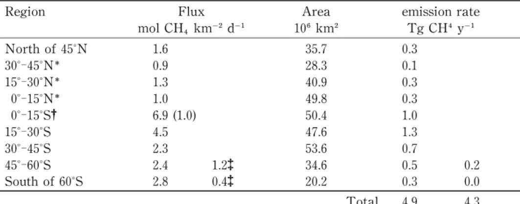
Bange et al.,1994］. The western part of the Sea of Okhotsk can be divided into 3 areas (Fig.2);in the central region of the Sea of Okhotsk, with depths deeper than 1000 m (section A),northwestern continental shelf region (sections F,G,and H), and east Sakhalin Shelf region (sections B, C, D, and E). Along section A, the methane flux (1.6 mol CH km d ) was somewhat larger than those (0.3 to 6.9 mol CH km d ) of the open ocean［Kiene, 1992;Bange et al. , 1994］. The northwestern continental shelf region, where methane is released from sedimentary sources, showed higher methane flux values (2.1 to 2.9 mol CH km d ) than those of section A. In the northeastern Sakhalin Shelf region, the methane flux (5.8 to 12.2 mol CH km d ) was remark- ably high.

The emission rate of methane was calculated to be 0.004 to 0.008 Tg CH y in the shelf northeast of Sakhalin affected by thermogenic sources, 0.003 to 0.005 Tg CH y in the area of the northwestern continental shelf affected by sedimentary sources, and 0.004 Tg CH y in the central region (Tables 2 ‑3). On the assumption of an average wind velocity of 7 m s throughout the year, Lammers et al.［1995 ］estimated a

Fig.15.Methane concentration against salinity in water over the northwestern continental shelf (section F average and station 1 to 4)in June‑ July 2000.

(14)

methane flux of 0.13 Tg CH y in the Sea of Okhotsk on the basis of measurements on the shelf northeast of Sakhalin in winter and summer.

By calculating averages for each region,the emission rate in the western Sea of Okhotsk (0.78× 10 km ,〜55% of total)was estimated to be 0.014 Tg CH y in boreal summer. In comparison with the results of Lammers et al.［1995 ］, we observed both relatively low supersaturation of methane in surface water stood on wide-ranging observations and smaller wind speeds based on objective analysis (Table 2).

Methane and freshwater originating from the Amur River control the sea-air methane flux in the western Sea of Okhotsk,which is supposed to vary greatly on a time scale from months to

years. Therefore, repeated measurements are necessary in order to estimate more precisely the annual methane flux in the Sea of Okhotsk.

Along the east coast of Sakhalin, the methane flux at stations close to land ( ＜〜100 m, Fig.16) was generally larger than those in the deeper shelf east of Sakhalin. As mentioned above, thermogenic methane was effectively transported to the surface by tidal mixing.

Therefore,tidal mixing plays an important role in increasing the methane flux over the shelf east of Sakhalin. On the basis of high methane concentrations observed below the ice cover in March 1991,Lammers et al.［1995 ］suggested that the seasonal ice cover in the Sea of Okhotsk induces a peak flux of accumulated methane as it

Table 2.Surface methane concentrations, methane saturation, wind speed, and air-sea flux at each location in the western Sea of Okhotsk.

Region Cruise Section Methane concentration Methane saturation Wind speed Air-sea flux 〃

year (nmol kg ) (%) (m s ) (mol CH km d )

mean range mean range mean range mean range Central 1998 A 3.6± 0.6 3.0‑4.6 139 116 ‑175 4.8 4.1‑5.2 1.6 0.68‑3.4 7 Shelf Northeast of

Sakhalin 1998 B 7.3± 8.0 2.7‑25.1 278 112‑905 3.7 2.7‑4.1 3.5 0.36‑11 7 1999 B 5.0± 1.9 3.2‑8.2 191 127 ‑313 6.2 6.2‑6.2 7 2 ‑16 5 2000 B 5.6± 0.8 4.8‑7.1 196 165 ‑251 5.1 5.0‑5.4 4.9 3.4‑7.7 7 1998 C 9.9±11.6 2.8‑41.5 390 120 ‑1523 3.7 3.4‑4.1 7.3 0.57‑33 10 1999 C 5.1± 4.0 3.2‑8.3 197 128 ‑316 6.1 5.6‑6.7 9.3 2.5‑25 7 2000 C 38.1±32.6 4.0‑79.8 1192 129‑ 2440 4.8 4.5‑5.2 43 1.4‑88 6 1998 D 9.3± 5.5 3.5‑14.9 349 144 ‑564 3.7 3.1‑4.5 6.3 1.8‑13 4 1999 D 7.6± 5.4 3.1‑13.6 293 124 ‑507 6.7 6.1‑7.3 12 2.5‑30 3 2000 D 6.9± 2.2 4.1‑10.4 212 127 ‑313 4.9 4.7‑5.1 4.9 1.3‑8.8 5 1999 E 4.1± 0.9 3.4‑6.3 144 116 ‑229 6.2 5.7‑6.6 3.2 1.3‑8.1 10 2000 E 5.3± 0.7 4.3‑6.5 169 127 ‑217 5.0 4.7‑5.1 3.3 1.4‑5.4 11

weighted average: 8.6 Northwestern

continental shelf 1999 F 3.7± 0.4 3.1‑4.4 138 117‑152 5.4 3.7‑6.3 2.1 0.78‑3.3 10 2000 F 4.4± 0.6 3.8‑5.7 146 129‑ 182 4.2 2.6‑5.1 1.5 0.47‑4.1 10 1999 G 4.4± 0.4 4.1‑4.7 155 147 ‑163 5.0 4.4‑5.7 2.8 2.6‑2.9 2 2000 G 8.2± 4.7 4.5‑10.9 283 156 ‑377 4.4 3.7‑4.7 7.9 2.5‑11.0 3 1999 H 3.7± 0.4 3.4‑4.1 136 126 ‑147 5.2 4.4‑5.5 1.8 1.6‑2.0 3 2000 H 4.9± 1.1 3.8‑6.1 168 128 ‑211 4.4 3.9‑4.6 2.6 1.1‑4.7 3

weighted average: 2.5

Table 3.Emission rate of methane in the western Sea of Okhotsk in boreal summer Area code Area Emission rate of methane

(km ) (TgCH y )

1998 1999 2000 mean Shelf northeast of Sakhalin NE 0.11×10 0.004 0.005 0.008 0.006 Northwestern continental shelf NW 0.25×10 − 0.003 0.005 0.004

Central CE 0.42×10 0.004 − − 0.004

Total 0.78×10 − − − 0.014

＊South of Sakhalin the flux was considered to be equal to that in the shelf northeast of Sakhalin (see Figures 2-7).

Osamu Y

(15)

retreats. However, our results suggest that because stratification remains in areas deeper than 50 m, the methane-rich water hardly venti- lates, which fact could cause less methane flux than expected from the high methane concentrations below the surface. It is, of course, necessary to examine the seasonal variation in surface methane concentration in order to discuss the sea-air methane flux further in detail.

2.3.4 Vertical and lateral transport of meth ane off east Sakhalin

-

During the southward flow of the East Sakhalin

Current,the methane concentration in the surface water generally increased from section B to section C (Fig.9). The methane flux between the sea and the air was not large enough to establish equilibrium during the southward flow,which had an average speed of 0.3‑ 0.4 m s ［Ohshima et al., 2002］. By assuming a flow speed of 0.3 m s and using the average methane flux of the 2 sections (Table 1), we calculated the amount of methane added to the surface between sections B and C to be 4 nmol kg in August ‑September 1998,2 nmol kg in July‑August 1999, and 40 nmol kg in June‑July 2000. If the methane was transported by vertical diffusion, then the methane flux, Q, from the subsurface to the surface mixed layer is calculated as:

Q＝−D ΔC

ΔZ , (4)

where Dz is the vertical diffusion coefficient and (ΔC/ΔZ) is the vertical gradient of the methane concentration. The diffusion coefficient was calculated to be 0.1‑0.4 cm s in August‑ September 1998 and July‑August 1999,and about 1 order of magnitude larger ( 〜1 cm s )in June‑ July 2000. This analysis may be too simple for a discussion of the vertical transport of methane off east Sakhalin,but it clearly shows the decreasing effect of stratification due to freshwater inputs from the Amur River on the methane transport from the subsurface to the surface mixed layer.

To determine the oxidation rate of methane,we obtained the amount of methane in a water column by integrated methane concentration from the surface to the bottom along section C and D.

Then we calculated the whole amount of methane in a 1‑m strip of water from 143.5°to 144.8° E along section C, and from 144.5°to 149.0° E along section D (Table 4), because the East Sakhalin Current flows south mainly and to southeast above a gently sloping bottom ［Ohshima et al., 2002;Mizuta et al., 2003］and no linear relationship between methane concentration and temperature indicating diffusion are plotted in Fig.17.

From the amount of methane emitted to the atmosphere over 16 days,and by assuming a flow speed of 0.3 m s between the 2 sections and a first-order reaction, we estimated the half-life of

Fig.16.Longitudinal distributions of methane flux between the sea and the air over the shelf northeast of Sakhalin.

(16)

methane oxidation as 15 days in July‑August 1998 and 30 days in June‑July 2000. We did not estimate the half-life in July‑August 1999,since only a few data were obtained along section C. High rates of microbial methane oxidation in seawater were reported in areas that contain high methane

［Nakamura et al., 1994;Valentine et al., 2001］. Our results are compatible with those previous results. In order to use methane as a quantitative chemical tracer,it will be necessary to exper- imentally determine the biological oxidation rates of methane just after the collection of sample seawater.

2.4 Summary

In the Joint Japanese ―Russian―U.S. Study of the Sea of Okhotsk, oceanic methane concentrations were measured in order to examine the distribution of methane, variations in its concentration, and the sea-air methane flux in the western part of the Sea of Okhotsk in July‑August 1998, August‑September 1999, and June ‑July 2000. Contrary to the earlier report in the Man-

dovi estuary,Goa,India［Jayakumar et al.,2001］, fresh eater inputs from the Amur River showed relatively low concentration of methane. In waters over the shelf northeast of Sakhalin, anomalously high concentrations occurred in the near-bottom water (26.6 ‑26.8 σ) at the eastern edge of the broad shelf ( 〜200 m), owing to methane seepage from an underlying oil field

［Ginsburg et al., 1993;Lammers et al., 1995］. This allowed us to trace the East Sakhalin Cur- rent flowing southward along the coast and southeastward away from Sakhalin on a time scale of a few months. In the area with depths of 50 ‑200 m,freshwater inputs from the Amur River led to strong stratification, which restricted the methane-rich subsurface water from ventilating.

The coefficient of vertical diffusion from the subsurface to the surface mixed layer in the same area was calculated to be 0.1 ‑0.4 cm s with a freshwater cap, and about 1 order of magnitude smaller without a freshwater cap. Along the east Sakhalin coast where the depth is shallower (＜〜100 m), tidal currents enhanced the vertical transport of methane-rich water to the surface.

In the area of the northwestern continental shelf,methane was discharged from sediments to the water column,especially off the east coast of Sakhalin,where a lot of organic matter from the Amur River is accumulated without decomposition. In the central region of the Sea of Okhotsk, the methane concentration showed a broad maximum in water with a density of 26.6‑26.8 σ, owing to in situ production of methane, as found in the open oceans and in the southeastward arm of the East Sakhalin Current.

In the area of the shelf northeast of Sakhalin (0.11×10 km ),which is affected by thermogenic sources, the emission rate of methane was calculated to be 0.006 Tg CH y . In the northwest- Table 4.Amount of methane (g)in whole water column

in a l-m strip along sections C and D.

Section Latitude 1998 1999 2000

C 143.5°‑144.8°E 41,308 9,509 43,687 D 144.5°‑149.0°E 14,999 − 25,928

From sections C to D,the amount of methane emitted to the atmosphere was estimated to be 441 g CH in July‑August 1998 and 1972 g CH in June ‑July 2000.

Fig.17.Methane concentration vs.water temperature along section C to D in 1998 and 2000.

Osamu Y

(17)

ern continental shelf region (0.25 × 10 km ), which is affected by sedimentary sources, it was calculated to be 0.004 Tg CH y . In the central region of the Sea of Okhotsk (0.42 × 10 km ), where the area has a larger flux of methane than in the open oceans, it was estimated to be 0.004 Tg CH y . Thus,in the western Sea of Okhot- sk (0.78× 10 km , 55% of total), the emission rate of methane was calculated to be 0.014 Tg CH y in boreal summer.

By taking into account the methane budget along section C from 143.5°to 146.0° E and along section D from 144.5°to 149.0° E,we estimated the half-life of methane oxidation to be about a month (15‑30 days) by assuming the first order reaction of methane.

Chapter 3 Methane in the South Pacific and Southern Ocean in austral summer 2001‑2002

3.1 Introduction

To estimate an accurate amount of the methane exchange from ocean to atmosphere, it is necessary to examine process controlling surface methane concentration widely and vertically.

Several reports showed that vertical profile of methane concentration has the maximum at subsurface layer in the Ocean［e.g.,Scranton and Brewer, 1977;Watanabe et al. , 1995;Kelley and Jeffrey, 2002］. There have been made some suggestion about the origin of the subsurface maximum, advection from nearby sources in shelf sediments, diffusion and /or advection from local anoxic environments, and in situ production by methanogenic bacteria,presumably in association with suspended particulate material. In the open ocean, some observations indicated that biogenic methane production occurred in the subsurface layer. The methanogenic bacteria produce methane in the seawater, but they cannot survive under any traces of oxygen. Therefore, these bacteria are thought to probably live in the anaerobic microenvironments supplied by organic particles or guts of zooplankton［e.g.,Alldredge and Cohen, 1987］. The methanogens also appear to be zooplankton species-specific ［de Angelis and Lee, 1994］, which further contributes to the lack

of a consistent correlation between seawater methane concentration and measured biological parameters［Burke et al. , 1983］. Recently, it is reported that some amount of methane is released by zooplankton-phytoplankton co-culture in the laboratory. But, there are only a few data that prove environmental subsurface methane production. Methane production in surface seawater is balanced by microbial oxidation［ Ward et al., 1987;Jones, 1991］and sea-air exchange. Open ocean turnover times with respect to biological oxidation are of the order of year ［Ward et al., 1987;Jones, 1991;Kiene, 1991］, which suggests that sea-air exchange is the major sink for seawater methane. So, this study investigates in detail profile of methane concentration and distribution in the water column in the South Pacific as an open ocean and the Southern Ocean as one of the most biologically productive regions characterized by large scale zooplankton such as Antarctic Krill and Sulpa (Fig.18). Moreover, observations are performed to address the temporal variation of oceanic methane at the same transect in the Southern Ocean, aboard the R/ V Hakuho Maru and the R/ V Tangaroa.

3.2 Materials and Methods

We collected about 1000 seawater samples at hydrographic stations in the South Pacific along 160°W and in the Southern Ocean along 140° E (dots in Fig.1), using the R/V Hakuho Maru of

Fig.18.The conceptual scheme of the methane production from the phytoplankton-zooplankton.

(18)

the Ocean Research Institute, University of Tokyo as KH‑01‑3 cruise (December 2001 in the South Pacific and January 2002 in the Southern Ocean) and using R/V Tangaroa of National Institute of Water and Atmospheric Research, New Zealand as the 43rd Japanese Antarctic Research Expedition Marine Science Cruise (Feb- ruary 2002 in the Southern Ocean along the same transect of Hakuho Maru Cruise).

The surface seawater samples were collected in a 1‑L bucket, and other samples were collected from 5‑25 depths from the surface ( 〜10 m)to the bottom in 12‑L Niskin bottles. Each sample was carefully subsampled into a 30 ‑mL glass vial so as to avoid contamination by air. The seawater samples were poisoned with 20 μL of mercuric chloride solution［Tilbrook and Karl, 1995;

Watanabe et al., 1995］, and then the vials were closed with rubber and aluminum caps. They were stored in a cool, dark place until the gas chromatographic analysis of methane on board or in our laboratory on land.

The analytical method was equal to that in the study for the Sea of Okhotsk (see Chapter 2).

The standard gases used contained 2.02,19.6,and 38.4 ppmv (Nippon Sanso Co.Ltd) of methane in pure nitrogen.

3.3 Results and Discussion

3.3.1 Methane in the South Pacific

3.3.1.1 Methane distribution and saturation At each station,the surface methane was supersaturated with respect to the methane in the air (Fig.19). The equatorial region had higher saturation ratio than more southerly sites. The surface methane concentration increased by 1 nmol

kg at 0°and 5°S as compared with those in the bulk of mixed layer. Watanabe et al.［1995］ reported that the saturation ration ranged from 109‑162% in the North Pacific (0 ‑40°N along 165°

E). In the western Equatorial Pacific, where is the area known as the western Pacific warm pool with low macro-nutrients and low salinity, they reported lower methane concentration ( 〜2.5 nmol kg ). The relatively high methane concentration in the present work is likely to be associated with high biological activity and methane production due to the equatorial upwelling. The saturation ratio became lowest near 10° S, and gradually increase with going to the south (Fig.

20). This is the pattern similar to that observed by Bates［1996］and Kelley and Jeffrey ［2002］.

The maximum concentration of methane in the subsurface layer or in the mixed layer was within the range from 2.9 to 4 nmol kg along 160°W (Fig.20). The vertical distribution of methane concentration differed from those of biological parameters such as chlorophyll a, macro- nutrients,and so on. This was mainly caused by processes of methane production in seawater as mentioned above. Kelley and Jeffrey ［2001］observed subsurface maxing, generally at the base

Fig.19.Longitudinal distribution of methane saturation ratio in South Pacific.

Fig.20.Distribution of methane concentration in the South Pacific (nmol kg ).Note the change in scales for surface 200 m.The numeral of most upper shows the methane saturation ratio (%).

Osamu Y

(19)

of the thermocline, in dissolved methane concentration at every site along the transect. How- ever, our results sometimes showed no clear maximum concentration of methane in the subsurface layer.

3.3.1.2 The increase in the marine surface methane for past of 30 years

Bange et al.［1994 ］examined diurnal variation in oceanic methane in the south central North Sea, and found little change. Until now, there are only a few works which focused on seasonal and year-to-year change in oceanic methane.

The observation of the surface water methane in the ocean was carried out in the beginning in 1970ʼs,and its saturation ratio of 130% was reported［Ehhalt, 1974］. Atmospheric methane concentration in those days was〜1.4 ppmv,methane concentration in the air in equilibrium to the surface water in oceanic region was 〜1.8 ppmv.

In this study,the saturation ratio is calculated as the atmospheric methane concentration is to be 1.8 ppmv. The saturation ratio shown here had over 100% (supersaturated), and the possibility was shown in which methane concentration of the surface water has increased over years in response to the increase of atmospheric methane.

3.3.2 Methane in the Southern Ocean

3.3.2.1 Oceanic structure in the Southern Ocean

In the Southern Ocean, major fronts were con- firmed［Preliminary Report of The Hakuho Maru Cruise KH‑01‑3,2003;Preliminary Report on the 43rd Japanese Antarctic Research Expedition Marine Science Cruise by Research Vessel Tangar- oa, 2002］in January 2002 (Fig.21) and in Febru- ary 2002 (Fig.22). Figs.21 and 22 show that the each oceanic structure has not largely changed during the period from January 2002 to February 2002.

Around 49°to 49.5°S,a steep horizontal gradient in surface temperature (Fig.21) and salinity was observed (data not shown)in January 2002. This was recognized as the Subantarctic Front, which is generally defined by the maximum temperature gradient in the range 3°to 8° C at 100 to 400 m

depth［Belkin and Gordon, 1996］. The Polar Front is commonly defined as the northernmost extent of temperature minimum water with temperatures less than 2°C at 200 m depth［Belkin and Cordon, 1996］. During our cruise, these features were recognized around 54° S. South of the Polar Front, cold fresh surface waters are known as Antarctic Surface Water.

Orsi et al.［1995］identified another deep front south of the Polar Front that coincides with the southern limit of temperature maximum water warmer than 1.8°C and is known as the Southern Antarctic Circumpolar Current Front. Rintoul and Bullister［1999］found this front to be about 63°S along 140°E, corresponding to the southern- most maximum of eastward transport. The existence of the Southern Antarctic Circumpolar Current Front in January and February was around 63°and 65°S respectively. An upwelling of water with warmer temperature ( ＞1°C) and higher salinity (34.5) was observed around 64° S, probably forming the Antarctic Divergence.

The Permanently Open Ocean Zone (POOZ) is commonly defined by waters between the Polar Front and the Southern Antarctic Circumpolar

Fig.21.Distribution of temperature in January.

Fig.22.Distribution of temperature in February.

(20)

Current Front. South of the Southern Antarctic Circumpolar Current Front, where are known as Seasonal Ice Zone (SIZ). In this paper,it mainly argues in north and south in the Southern Antarc- tic Circumpolar Current Front (i.e. POOZ and SIZ), because there is no data from 54° S to the north in the observation in February.

Antarctic Bottom Water is a dense water mass that forms around some areas of the Antarctic coast and sinks to abyssal depths along the Ant- arctic continental slope［Orsi et al., 1999］. Rintoul and Bullister［1999］showed that Antarc- tic Bottom Water along 140°E was rich in CFCs at depths of＞3000 m. The high concentrations of CFCs found in Antarctic Bottom Water suggested that production and export of Antarctic Bottom Water is an efficient mechanism for transporting surface waters to the deep sea.

3.3.2.2 High methane concentration in the sur face layer

-

We divided the area south of the Polar Front into two zones, POOZ and SIZ. In the former zone,the maximum methane concentrations were observed in the mixed layer and they are almost the same value of 3.7±0.6 nmol kg (Figs.23‑25).

In the latter zone,the maximum methane concentration was also observed in the mixed layer,and methane concentration was apparently associated with chlorophyll a concentration (Figs.26 and 27).

Concentration of chlorophyll a is controlled by photosynthetic process and zooplankton grazing and degradation of the organic matter ［Oudot et al., 2002］. As mentioned above methane is produced by methanogenic bacteria and meth-

anogen associated with suspended particles,fecal pellets, and guts of zooplankton. The relationship between methane concentration and quan- tity/grazing rate of zooplankton should be considered, because the phytoplankton does not form the methane directly. Unfortunately, at present data of the zooplankton are not available.

Fig.23.Distribution of methane concentration in Jan- uary from 43°to 66°S (nmol kg ).

Fig.25.Distribution of methane concentration in Feb- ruary from 54°to 66°S (nmol kg ).

Fig.24.As for Figure 23 except in from 54°to 66°S.

Fig.26.Vertical profiles of chlorophyll a concentration upper 350 m. Square and diamond represent the data in January and February respectively.

Osamu Y

(21)

In the POOZ and SIZ, the methane concentration below the mixed layer decreased drastically to the level of 1 nmol kg (Figs.23‑25),therefore we did not found any subsurface maximum methane concentrations south of the Polar Front.

Holmes et al.［2000］suggested methane production in organic rich particles at the pycnocline to account for the subsurface maximum. Taking into discussions about methane production and oxidation［Holmes et al. , 2000; Ward and Kilpatrick, 1993;Karl and Tilbrook, 1994 ］, we examined the vertical profiles of methane concentration at〜27.1 σ which is the density at the base of mixed layer in south of the Polar Front (Fig.28). Around this σθthe methane concentration changed steeply at every site along the transects. This support the mechanism suggested by Holmes et al.［2000］.

3.3.2.3 Methane saturation and sea-air flux The methane saturation ratio was shown in

Figs.29 and 30 in the each station. In the observation in January, all the station was supersaturated, and the methane discharged to the atmosphere from the ocean, and in the observation in February, some station was undersaturation,and it seemed to absorb methane from the atmosphere.

The flux in the observation in January was calculated by using equation (1),(2),and (4). The wind speed was the average wind speed measured by the shipʼs anemometer during the sampling period. The high rate flux was observed in the station where a good correlation between chlorophyll a concentration and methane concentration.

As mentioned in 3.3,the relative error associated with kw determined by equation (4) is about 25%, assuming a 10% error on the Schmidt number［Wanninkhof, 1992］and using the measured variability in the wind speeds while sampling.

About 40% error is contained as a whole.

Fig.28.Distribution of σ in January. Fig.30.As for Figure 29 except in February.

Fig.29.Methane saturation ratio (%) with distribution in January.

Fig.27.Methane concentration vs.chlorophyll a from 62°S to 64°S. Blue square and red diamond represent the data in January and February respectively.