A Study on Multi-Agent Systems for Stable Matching

A Study on Multi‑Agent Systems for Stable Matching

著者 モハマド シャキリン ビン ラムリ

著者別表示 Mohd Syakirin Bin Ramli journal or

publication title

博士論文要旨Abstract 学位授与番号 13301甲第4316号

学位名 博士（工学）

学位授与年月日 2015‑09‑28

URL http://hdl.handle.net/2297/43854

Abstract For Dissertation

A Study on Multi-Agent Systems for Stable Matching

Division of Electrical Engineering and Computer Science Graduate School of Natural Science & Technology

Kanazawa University

Intelligent Systems and Information Mathematics

Student Number: 1223112006

Mohd Syakirin bin Ramli

Chief Advisor: Shigeru YAMAMOTO, Prof.Dr.

2 STABILITY THEORY

1 Motivation and Objectives

The stable marriage problem (SMP) is a combinatorial optimization problem of finding a stable matching between two sets, namely men and women. Each man and woman has their own set of preference lists in which they rank orderly their preferred partners. With this information, the aim of solving the matching problem is to establish a stable partnership without the blocking pairs.

The terminology of SMP was first coined in year 1962 by David Gale and Lyod Shapley in their seminal work of [1]. They introduced a sequential algorithm (as from now on we refer it as G-S algorithm) to establish matching between two bi- partite sets, in consideration of matching students with their appropriate colleges, or in the marriage situation per se. The algorithm works by one side of the divides to make the proposal, while the other evaluates either to accept or reject the said proposal. The proposing iteration continues as long as there exists proposer which has yet to be matched with his/her stable partners.

The G-S algorithm works flawlessly to attain stable matching between these two sets without the blocking pairs. However, it only uses partial information from the preference lists. Therefore, there are possibilities that other matching might yield to better matching results suppose full information is used. Moreover, the G- S algorithm favors proposer than the receiver. Hence, the final matching attained by the G-S algorithm will be optimal to the men (if they are the proposer) over the women. These phenomena is commonly known as the men-optimal, women- pessimal situation.

The way this algorithm works in sequential manner limits the usage of all the information available in the preference lists. Therefore, in this dissertation we aim to emulate the strategies given by the G-S algorithm, but to introduce dynamical approach in attaining stable matching between the bipartite sets. In the following, we state the main objectives which motivate us in our investigation of the stable marriage problem.

The objectives of this work are as follows:

• To investigate the potential of treating a discrete optimization problem through solving the sets of di↵erential equations in the multi-agents formulation.

• To identify and formulate suitable cost function that best interpret the prefer- ence lists of both men and women.

• To attain dynamically stable matching between men and women.

2 Stability Theory

Consider the autonomous system of

˙

x = f (x(t)) (1)

where f : D ! R

ⁿ

is locally Lipschitz map from domain D ⇢ R

ⁿ

into R

ⁿ

. The sys-

tem (1) is said to be continuous and smooth, since the right hand side is continuous.

2 STABILITY THEORY

On the other hand, let the di↵erential equation with discontinuous right hand side be represented by a di↵erential inclusion

˙

x 2

^a.e.

K { f (x, t) } (2)

where K { f (x, t) } is the Filippov’s di↵erential inclusion and a.e. is the abbreviation for “almost everywhere”.

Definition 1 (Filippov solution [2, 3]) . A vector function x( · ) is called a solution of (2) on [t

0

, t

1

] if x( · ) is absolutely continuous on [t

0

, t

1

] and for almost all t 2 [t

0

, t

1

]

˙

x 2 K { f (x, t) } (3)

where

K { f (x, t) } = \

_>0µ(D)=0

\ co f (B(x, ) D, t) (4)

where co means the closed convex hull; B(x , ) is a closed neighborhood of x;

D is an arbitrary set in R

ⁿ

; µ is n dimensional Lebesgue measure. Hence, \

µ(N)=0

means the intersection over all sets D of Lebesgue measure zero.

2.1 Lyapunov Stability

To investigate the stability of a given dynamical system, we may analyze the sta- bility of the solutions of its di↵erential equations near to a point of equilibrium.

Hence, by ensuring that the stability conditions are satisfied, then we can conclude about the behavior of those system at this point. The following lemmas provide us with essential tools in analyzing the stability of the dynamical system near its equilibrium points.

Lemma 1 (Lyapunov’s second method for stability) . Assume that the system (1) has an equilibrium point at x = x

0

. Then, the system is asymptotically stable in the sense of Lyapunov if and only if, there exist a Lyapunov function V(x) : R

ⁿ

! R such that

• V(x) > 0 for all x , x

0

and V(x

0

) = 0,

• V(x) ˙ < 0 for all x , x

0

and ˙ V(x

0

) = 0.

Suppose the right-hand-side of (1) is non-smooth (i.e., equation (2)), then the following lemma provides the generalized form of Lemma 1 to discuss the stability of the non-smooth dynamic.

Lemma 2 (Generalized Lyapunov Theorem). Given that (2) is discontinuous on the right-hand-side, and has an equilibrium point x = x

0

. Then, if there exists

• a V : R

ⁿ

! R , V(x

0

) = 0, V(x) > 0, 8 x , 0, such that V(x(t)) is absolutely continuous on [t, 1 ),

• with d

dt [V(x(t))] < ✏ < 0 a.e. on { t | x(t) , x

0

} ,

then x converge to x

0

in finite time. Thus, the system (2) is generally asymptotically stable in the sense of Lyapunov.

Proof. See Theorem 2 in [3] for the complete proof. ⇤

3 PROBLEM FORMULATION

3 Problem Formulation

3.1 Gale and Shapley Algorithm

We assume that there exists sets of men M := { m

1

, m

2

, . . . , m

P

} , and women W :=

{ w

₁

, w

₂

, . . . , w

_P

} with P is the number of pairs. Each of the individuals in these two sets rank orderly their preferred partners in the preference lists. Let us denote the man m is the current man proposing to the woman w in his preference list. Also, if the proposed woman w is already engaged, we denote her current partner as ¯ m.

We denote ¯ w as the next-woman to be proposed from of the man m’s preference list.

The procedure of the G-S algorithm [1] is presented in Algorithm 1.

Algorithm 1 Gale & Shapley Algorithm (Men-proposer)

1: procedure S table M atching (m , w )

2: Initialize all men and women to be free

3: while 9 free m do

4: w = m’s highest ranked woman to whom he has not yet proposed

5: if w is free then

6: m = p

M

(w) & w = p

M

(m)

7: (m, w) ! M . m, w become partner

8: else if w is already engaged with ¯ m then

9: if m precedes ¯ m in w’s preference list then

10: w = p

M

(m)

11: (m, w) ! M . w choose new partner

12: m ¯ becomes free

13: else

14: w = p

M

( ¯ m) remain engaged

15: ( ¯ m, w) ! M . ( ¯ m, w) remain partner

16: m proposes to ¯ w in his preference list

17: end if

18: end if

19: end while

20: Final matching is established.

21: end procedure

This algorithm is guaranteed to terminate at O(P log P) iterations[4], and upon termination, stable pairs M will be established. The stable pairs established in M is said to be Men-Optimal, Women-Pessimal since the men are the first proposing to the women. The results will be the opposite if women is the first party to propose [1, 5].

Notice that G-S algorithm utilizes the sequential steps of optimizing in seeking

for the stable pairs between the bipartite sets. In the following chapters, we attempt

to address the same optimization problem as before, but utilize the multi-agent sys-

tem to achieve the objective.

3 PROBLEM FORMULATION

3.2 Agents Dynamics

We consider N agents moving in an n dimensional Euclidean space. Each of the agents is described by a single integrator as

˙

x

i

= u

i

, (5)

where x

i

2 R

ⁿ

is the position vector of agent i and u

i

2 R

ⁿ

is the (velocity) control input to be designed. To represent N agents, the total state and control vectors are defined as

x = 2 66666 66664

x

1

.. . x

N

3 77777

77775 2 R

^nN

and u =

2 66666 66664

u

1

.. . u

N

3 77777

77775 2 R

^nN

, (6)

respectively. We further rewrite the total system dynamic in the form

˙

x = u. (7)

The group center that is the virtual center state can be obtained by considering the average of all positions as

x

c

= 1 N

X

N

i=1

x

i

. (8)

It is also assumed that the desired state trajectory x

d

2 R

ⁿ

for the group center x

c

can be achieved by u

d

2 R

ⁿ

, that is

˙

x

d

= u

d

. (9)

3.3 Dynamical Stable Marriage Problem

In this section, we introduce the the terminology of the dynamical stable marriage problem. For the case of the dynamical stable marriage problem, we aim to find the optimum stable matching between the bipartite sets by using the dynamic of the multi-agent systems.

We consider a group of agents I = { 1, 2, . . . , N } and the corresponding positions X = { x

1

, x

2

. . . , x

N

} , where x

i

is defined in (5). We assume that I = M [ W and M \ W = ; . Furthermore, we assume that P satisfies N = 2P. In addition, let the odd numbering agents belong to the men set and the even numbering agents belong to the women set, respectively. That is,

i 2 M $ i 2 I

M

:= { 1, 3, . . . , N 1 }

i 2 W $ i 2 I

W

:= { 2, 4, . . . , N } . (10)

The following definition provides the physical interpretation of the dynamical stable

matching.

3 PROBLEM FORMULATION

Definition 2 (Dynamical Stable Matching). For the agent x

i

, we define an index set denoting opposite gender and same gender as follows.

J

i

=

( I

W

if i 2 M

I

M

if i 2 W , K

i

=

( I

M

if i 2 M

I

W

if i 2 W . (11) The agents i 2 I are said to dynamically achieve stable matching if

(a) for the stable partner j

^⇤

2 J

i

of i, (i.e., j

^⇤

:= p

M

(i) 7! (i, j

^⇤

) 2 M), then lim

t!1

k x

j^⇤

(t) x

i

(t) k = 0.

(b) for k 2 K

i

there exists t

0

> 0 such that k x

k

(t) x

i

(t) k d for all t > t

0

. (c) the center trajectory x

c

satisfies lim

t!1

k x

c

(t) x

d

(t) k = 0, for the desired trajectory x

d

.

To achieve the dynamical stable matching, we use the weighted degree w

_{i j}

de- fined as follows:

Definition 3 (Weighted Degree) . The weighted degree w

_{i j}

is defined by using the preference rank p

i j

as

w

_{i j}

= 8 >>><

>>>:

2

|J

i

| ( |J

i

| + 1)

⇣ |J

i

| p

i j

+ 1 ⌘

if j 2 J

i

0 otherwise , (12)

where |J

i

| is the cardinality of J

i

.

3.4 Lyapunov Function Minimization

In designing the suitable control law for the dynamical stable matching, we utilize all information available in the preference list. We design a Lyapunov function to be minimized as

V(x) = V

T

(x) + V

c

(x), (13)

where V

T

(x) > 0 : R

^nN

! R and V

c

(x) > 0 : R

ⁿ

! R are defined to use a multiplier constant ⌫

_ik

> 0 2 R and the weighted degree w

_{i j}

as

V

T

(x) =

X

N

i=1

V

i

(x), (14)

V

i

(x) = exp X

j2Jⁱ

w

_{i j}

k x

j

x

i

k + X

k2Ki

⌫

_ik

(d k x

k

x

i

k )

²

1, (15) V

c

(x) = 1

2 k x

c

x

d

k

²

. (16)

The Lyapunov candidate V

T

is designed to take (a) and (b) in Def. 2 into con- sideration. Minimizing V

T

implies to solve an optimization problem:

minimize exp X

j2Jⁱ

w

_{i j}

k x

j

x

i

k

subject to k x

k

x

i

k d , 8 k 2 K

i

, i = 1 , 2 , . . . , N .

(17)

4 MAIN RESULTS

Meanwhile, the Lyapunov candidate V

c

is designed as the energy dissipation func- tion corresponding to the x

c

and x

d

to take (c) into consideration in Def. 2. The weight w

_{i j}

in (17) is defined in Def. 3.

Problem 1. For the dynamic of agent i in (5) and to use the weighted degree (12) obtained from the preferences list of men and women, design the appropriate control action u

i

such that the Lyapunov function (13) is minimized.

4 Main Results

4.1 Centralized Control

The following theorem provide the suitable control law to attain dynamical stable matching.

Theorem 1. (Fixed network stable matching theorem) For fixed network agents, starting from ⌦ = { x : V(x)  } , the dynamical stable matching is achieved under the state feedback control

u

i

= u

^{S M}_i

+ u

^c_i

(18)

u

^{S M}_i

= u

^a_i

+ u

^r_i

, (19)

u

^c_i

= k

^c

(x

i

x

d

) + u

d

, (20)

where u

^a_i

is the attraction of agent i with j 2 J

i

u

^a_i

= X

j2Ji

(a

i

b

i j

+ a

j

b

ji

)(x

j

x

i

) (21)

and u

^r_i

is the repulsion between agent i with k 2 K

i

u

^r_i

= X

k2Ki

(c

ik

+ c

ki

)(x

k

x

i

) , (22)

and k

^c

> 0 is an appropriate control gain and a

i

= exp X

j⁰2Ji

w

_{i j}0

k x

j⁰

x

i

k (23)

b

i j

= w

_{i j}

k x

j

x

i

k (24)

c

ik

= 2⌫

ik

1 d k x

k

x

i

k

!

. (25)

4.2 Decentralized Control

The proposed control law (19) for each agent i presented in Section 4.1 utilizes the

information from all agents. Due to the excess information, the calculated control

action tends to be very large. Hence, to overcome this problem we allow each agent

i to communicate only with its neighboring agents. As all agents tend to follow

the desired trajectory to achieve condition (c) in Def. 2, there will be more agents

within i’s sensing range, thus permitting for wider selection of agents to be matched

with.

4 MAIN RESULTS

Definition 4 (Neighboring Agents). Let R

g

be the distance sensing range of agent i.

Agent j is called a neighbor of agent i if it belongs to the set N

i

= n

j 2 I | r

i j

= k x

j

x

i

k  R

g

o . (26)

Due to limited communication between agents, we propose the decentralized control of the same form as (18) given by

u

i

= u

^{S M}_iN

+ u

^c_i

(27)

and in the vector form as

u = u

^{S M}_N

+ u

^c

(28)

where u

^{S M}_N

is denoted in (29) and u

^c

= (I

N

⌦ k

^c

)(x 1

N

⌦ x

d

) + 1

N

⌦ u

d

. The control law u

^{S M}_iN

in (27) is due to SMP and has the same form as (19), but with di↵erent control gains depending on the communication topology. In the vector form, it is recurrently defined as

u

^{S M}_N

= (L

^N

⌦ I

n

)x (29)

where L

^N

= L

^a_N

+ L

^r_N

with

L

^a_N

:= (l

^a,_{i j}^N

)

_N⇥N

= 8 >>>>>

< >>>>>

: P

j⁰2Ji\Ni

(a

^N_i

b

^N_{i j}0

+ a

^N_j0

b

^N_j0i

) if j = i

(a

^N_i

b

^N_{i j}

+ a

^N_j

b

^N_ji

) if j , i, j 2 J

i

\ N

i

0 otherwise,

L

^r_N

:= (l

^r,_{i j}^N

)

_N⇥N

= 8 >>>>>

< >>>>>

: P

k⁰2Ki\Ni

(c

^N_ik0

+ c

^N_k0i

) if k = i,

(c

^N_ik

+ c

^N_ki

) if k , i, k 2 K

i

\ N

i

0 otherwise.

The variables a

^N_i

, b

^N_{i j}

and c

^N_ik

of each agent i take the form of equation (23) but only their neighboring agents are taken into accounts. Here, we redefine (23) as

a

^N_i

= exp 0 BBBBB

B@ X

j⁰2Ji\Ni

w

_{i j}0

k x

j⁰

x

i

k 1 CCCCC CA b

^N_{i j}

= w

_{i j}

k x

j

x

i

k c

^N_ik

= 2⌫

ik

1 d

k x

k

x

i

k

! .

(30)

4.3 Discontinuous Dynamic

Due to the selection of control law (29), the total control dynamic (7) has discontin-

uous right-hand-side, hence it takes the di↵erential form of (3). Based on Def. 1 and

using (28) where f (x, t) = u = u

^{S M}_N

+ u

^c

, the di↵erential inclusion defined in (4) for

4 MAIN RESULTS

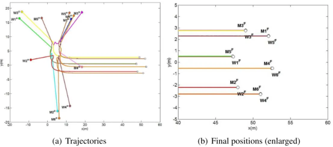
(a) Trajectories (b) Final positions (enlarged)

Figure 1: Agents trajectories in matching with their stable partners when we use the centralized control (18).

the discontinuous di↵erential equation of (3) can be calculated using the calculus in [3]. Hence, the total dynamic is obtained as

˙

x 2 K { f (x, t) } = K { u }

= K { u

^{S M}

} + K { u

^c

}

=

( u

^{S M}_N

+ u

^c

if 9

u

^c

otherwise,

(31)

where 9 , {8 i , 9 j 2 J

i

\ N

i

, 9 k 2 K

i

\ N

i

} . 4.3.1 Nonsmooth Stability Analysis

In similar form to (13), we use a suitable Lyapunov function candidate for the non- smooth system as

V(x) = V

T

(x) + V

c

(x) (32)

where

V

T

(x) =

X

N

i=1

V

i

(x) (33)

and V

c

(x) is defined in (16), respectively. However, slight modification in V

i

is needed so that J

i

is divided into two groups: neighbor J

i

\ N

i

and not neighbor J

i

\N

i

, and K

i

into K

i

\ N

i

and K

i

\N

i

, as well. That is,

V

i

(x) = exp 0 BBBBB

B@ X

j2Ji\Ni

w

_{i j}

k x

j

x

i

k 1 CCCCC

CA + exp

0 BBBBB

B@ X

j2Ji\Ni

w

_{i j}

R 1 CCCCC CA + X

k2Kⁱ\Nⁱ

⌫

_ik

(d k x

k

x

i

k )

²

+ X

k2Kⁱ\Nⁱ

⌫

_ik

(d R)

²

1 where V

i

( · ) 2 C

⁰

corresponds to the local Lyapunov function of agent i.

To achieve dynamical stable matching between agents with time-varying com-

munication topology, we propose the following theorem:

5 NUMERICAL EXAMPLE

(a) Trajectories (b) Final positions (enlarged)

Figure 2: Agents trajectories in matching with their stable partners when we use the decentralized control (27).

Theorem 2. (Time-varying network stable matching theorem) For time-varying network agents, starting from ⌦ = { x : V(x)  } , the dynamic stable matching between agents as defined in Def. 2 is generally asymptotically stable under the state feedback control u

i

(27) with appropriate control gain k

^c

.

5 Numerical Example

We consider a MAS consists of 12 agents (which constitute 6 stable pairs) in such they can be segregated into men and women’s sets. We denote the odd-numbering agents as belonging to the men set and the even-numbering agents are assigned to the opposite gender. Each of these agents ranks orderly their preferred partners as listed in Table 1. We assume that the individual agent has access to the information on the preference list of the other agents. We consider the movement of agents in the Euclidean space such that n = 2.

The positions of all agents at t = 0 were randomly initialized within [ 20m, 20m]

in both x-y coordinates. The desired trajectory dynamic was chosen as straight line given by x

d

(t) = [5t, 0]

^T

. Meanwhile, the desired distance separation between sta- ble pairs was set as d = 5m. The state feedback control gain and the multiplier constant were chosen as k

c

= 2 and ⌫

_i

= 10, respectively.

We first investigate the overall system’s behavior due to the centralized control law (18). Figure 1 shows the agents’ trajectories and their final positions, respec- tively. It can be seen that formation center converged to the desired trajectory which yield to the final matching of M = { m

1

w

₅

, m

2

w

₂

, m

3

w

₃

, m

4

w

₆

, m

5

w

₁

, m

6

w

₄

} satisfying all conditions in Def. 2.

Next, we tested the decentralized control law (27) to achieve the stable matching

in the multi-agent systems. In contrast to the centralized control structure, each

of the agents calculate its control action based on the information obtained from

the other agents which are within its sensing range. In this case, we choose the

sensing range of the agent i as R = 10m. Figure 2 shows the agent trajectories

and their final positions when we use the decentralized control law (27). The final

matching obtained by this control action is M = { m

1

w

₆

, m

2

w

₁

, m

3

w

₅

, m

4

w

₄

, m

5

w

₃

,

REFERENCES

m

6

w

₂

} .

6 Conclusion

Motivated by the Gale & Shapley seminal work, we investigated the potential of ac- quainting the SMP theory into MAS. Two control algorithms have been presented:

the centralized and decentralized control structures. Our results indicated that the total system is asymptotically stable in the sense of Lyapunov, but the final match- ing exhibited a number of blocking pairs. Hence, the final matching is unstable in terms of SMP stability theory.

A Example of Preference Lists

Table 1: Example of Men and Women Preference Lists for 6 pairs SMP Men’s List

1

^st

2

^nd

3

^rd

4

^th

5

^th

6

^th

m

1

w

₃

w

₆

w

₅

w

₁

w

₂

w

₄

m

2

w

₂

w

₁

w

₅

w

₆

w

₃

w

₄

m

3

w

₂

w

₃

w

₁

w

₆

w

₅

w

₄

m

4

w

₁

w

₃

w

₂

w

₄

w

₅

w

₆

m

5

w

₄

w

₆

w

₂

w

₃

w

₅

w

₁

m

6

w

₁

w

₆

w

₄

w

₂

w

₅

w

₃

Women’s List

1

^st

2

^nd

3

^rd

4

^th

5

^th

6

^th

w

₁

m

2

m

3

m

5

m

1

m

4

m

6

w

₂

m

6

m

4

m

2

m

3

m

5

m

1

w

₃

m

2

m

4

m

3

m

5

m

6

m

1

w

₄

m

5

m

4

m

1

m

6

m

3

m

2

w

₅

m

6

m

1

m

5

m

2

m

3

m

4

w

₆

m

3

m

4

m

2

m

6

m

5

m

1

References

[1] D. Gale and L. Shapley, “College admissions and the stability of marriage,”

The American Mathematical Monthly, vol. 69, no. 1, pp. 9–15, 1962.

[2] T. Ito, “A Filippov solution of a system of di↵erential equations with discontin- uous right-hand sides,” Economics Letters, vol. 4, no. 4, pp. 349–354, 1979.

[3] B. Paden and S. Sastry, “A calculus for computing Filippov’s di↵erential inclusion with application to the variable structure control of robot manipulators,” IEEE Transactions on Circuits and Systems, vol. 34, no. 1, pp.

73–82, Jan. 1987.

[4] L. B. Wilson, “An analysis of the stable marriage assignment algorithm,” BIT Numerical Mathematics, vol. 12, no. 4, pp. 569–575, Dec. 1972.

[5] D. Gusfield and R. W. Irving, The stable marriage problem: structure and

algorithms. The MIT Press, 1989.