The Impact of Trade on Economic Growth and Welfare with Heterogeneous Firms and Labor Market Frictions

(1)

The Impact of Trade on Economic Growth and Welfare with Heterogeneous Firms and Labor Market Frictions

NISHIYAMA Hiroyuki

^*

Institute for Policy Analysis and Social Innovation, University of Hyogo, Japan

GINTANI Ya suhiro

College of Economics, Kanto Gakuin University, Japan

TSUBOI Mizuki

Faculty of Economics and Business, Wako University, Japan

Abstract

Ca n tra de libera liza tion jointly ra ise long-run growth a nd welfa re? To a nswer this question, we develop a tra cta ble dyna mic tra de model with firm heterogeneity a nd fa ir wa ges. In sha rp contra st to sta nda rd Melitz models with endogenous growth, we do not a ssume a d hoc knowledge spillover. Instea d, defining GDP tha t is consistent with officia l sta tistics, we study the impa ct of tra de libera liza tion on economic growth a nd welfa re.

In the ba seline ca se where la bor ma rket frictions a re in isola tion, we a na lytica lly show tha t tra de libera liza tion ma y lea d to lower growth a nd deliver a welfa re loss due to severa l conflicting forces. We then simula te our model to demonstra te that there is a critica l intera ction between economic growth, welfa re, openness, a nd la bor ma rket frictions. For exa mple, in a less open economy with the lower level of la bor ma rket frictions, trade libera liza tion delivers a welfa re loss. This is a lso the ca se in a more open economy with the higher level of la bor ma rket frictions.

Keywords: Economic Growth; Welfa re; La bor Ma rket Frictions; Tra de Libera liza tion JEL Classification: F12, F16, F43

Source of Funding

Gra nts-in-Aid for Scientific Resea rch [KAKENHI: 18K01616 (H. Nishiya ma )].

*

(2)

1. Introduction

Can trade liberalization jointly raise long-run growth and welfare? To answer this question, we develop a tractable dynamic trade model with firm heterogeneity and fair wages. In sharp contrast to standard Melitz (2003) models with endogenous growth, such as Baldwin and Robert-Nicoud (2008) and Ourens (2016), we do not assume knowledge spillover. In- stead, defining GDP that is consistent with official statistics, we study the impact of trade liberalization (i.e., decreases in trade costs) on economic growth and welfare. In the baseline case where labor market frictions are in isolation, we analytically show that trade liberalization may lead to lower growth and welfare loss due to several conflicting forces. We then simulate our model to demonstrate that there is a critical interaction between economic growth, welfare, openness, and the level of labor market frictions. For example, in a less open economy with the lower level of labor market frictions, trade liberalization delivers a welfare loss. This is also the case in a more open economy with the higher level of labor market frictions. Table 1 summarizes our findings.

Degree of Openness

Level of Labor Market Friction Less Open More Open

Lower Welfare ↓ Welfare ↑

Higher Welfare ↑ Welfare ↓

Table 1: The Impact of Trade Liberalization on Welfare

The earlier papers that study the connections between economic growth and international trade assumed homogeneous firms.

¹

Thus, they cannot analyze reallocations of resources within industries that raise average industry productivity − an essential channel to understand the welfare effects of trade liberalization (Melitz, 2003). This limitation, however, was solved by the watershed contribution of Baldwin and Robert-Nicoud (2008); they integrate firm heterogeneity into those earlier frameworks featuring knowledge spillover. Therefore, they make it possible to study how trade-induced changes (i.e., reallocation effects) absent in earlier papers affect economic growth and welfare.

Subsequent research of Baldwin and Robert-Nicoud (2008) − henceforth BRN − revisit and extend their framework in a wide range of directions. Gustafsson and Segerstrom (2010) eliminate scale effects in BRN and show that the effects of trade liberalization on growth and welfare depend on how strong intertemporal knowledge spillovers are. Unel (2010) adds an assumption that the foreign contribution to local technology increases with the volume of trade to BRN, and finds that though trade liberalization increases average productivity, its effects on growth and welfare are ambiguous. Ourens (2016) revisits BRN and corrects their algebra mistakes, and figures out a new welfare channel missed in BRN. Fukuda (2019) also revisits BRN by introducing taxes on asset income, scientific research, and population

1

See, for example, Grossman and Helpman (1991), Rivera-Batiz and Romer (1991a; 1991b), Acemoglu

and Ventura (2002), and Ventura (2005).

(3)

growth.

²

While studies cited above have made key contributions to a better understanding of growth and welfare effects of trade liberalization with heterogeneous firms, there are yet three remaining shortcomings. First, they do not explicitly examine whether trade-induced higher growth is compatible with higher welfare; that is, they do not answer our research question posed above. Whether trade liberalization can jointly raise long-run growth and welfare is still unclear. Second, their models − including the original BRN − do not explain growth; they simply assume growth. Without assuming knowledge spillover, they cannot study growth and welfare effects of trade liberalization. We view their modeling of growth as an ad hoc, unsatisfactory story. Third, what they call growth is not growth; it is just changes in the number of firms (or varieties) and thus inconsistent with official statistics.

As GDP is not defined in their model, they implicitly assume a one-to-one correspondence between changes in GDP and the number of firms.

³

We do not think that this implicit assumption makes sense. As such, our goal is to rigorously define GDP in a dynamic trade model with heterogeneous firms by explicitly modeling financial markets based on Ghironi and Melitz (2005) and answer our research question by looking at a response of GDP and welfare to trade liberalization − but without relying on an ad hoc growth mechanism.

Moreover, we go beyond rather than just fixing three imperfections of above studies by introducing labor market frictions (or unemployment). As unemployment means an inefficient use of resources, a reduced living standard, and psychological distress, we all would agree that unemployment is an important consideration for growth and welfare. Fig. 1 makes our point: it shows an interaction between economic growth, openness, and unemployment among 37 OECD countries in 2017. As we can see, a look at only the link between growth and openness is misleading. In addition to these two elements, countries substantially differ according to their rate of unemployment. Thus, to fully understand the growth and welfare effects of trade liberalization, we take labor market outcomes into account. Since all studies cited above assume frictionless labor markets in which all workers are fully employed, they cannot analyze the trade-induced changes in labor market outcomes and their consequences on growth and welfare. For these reasons, based on Akerlof and Yellen (1990) and Egger and Kreickemeier (2009), we introduce fair wages as the source of labor market frictions.

⁴

Combined with the degree of openness, our model gives a richer picture to examine whether trade liberalization can jointly raise long-run growth and welfare.

Four patterns in Table 1 are due to several conflicting forces. Specifically, we first de-

2

The other follow-up studies focus on country asymmetries. Unel (2013) constructs a two-country asymmetric Melitz model in which technology adoption costs differ across countries, and demonstrates that trade liberalization may not improve the welfare in the country with higher technology adoption costs. Wu (2015) integrates multinational enterprises (MNEs) into a two-country asymmetric Melitz model without scale effects and finds a U-shaped relationship between growth (welfare) and trade costs. Naito (2017) studies the asymmetric version of BRN with respect to wages and the number of varieties, and discusses the growth and welfare effects of unilateral trade liberalization. Finally, Ourens (2020) develops a North-South version of BRN.

3

Another drawback is that they cannot study level effects.

4

See Felbermayr et al. (2011) for a Melitz model with search and matching frictions.

(4)

Figure 1: Growth rate, openness, and unemployment rate among 37 OECD countries in 2017. Openness (scaled logarithmically) is the sum of exports and imports of goods and services relative to GDP. Source:

Growth and openness are from Penn World Table 9.1 and unemployment from IMF World Economic Outlook Database April, 2020.

compose the impact of trade liberalization on growth into the following three: an increase in output per firm due to a rise in average productivity, a decrease in the mass of producing firms due to a rise in average productivity, and an increase in the mass of new entrants in anticipation of a larger profit. While the first and third lead to an increase in GDP, the second leads to a decrease in GDP. Thus, the net effect is ambiguous. Next, for welfare, in addition to these three channels, we have the fourth: an intertemporal optimal consumption choice of households. In response to trade liberalization, households save more and consume less in anticipation of a rise in expected dividend induced by an increase in new entrants.

This new channel being added, unlike Melitz (2003), trade liberalization can deliver a welfare loss in our model.

There are two closely related studies. First, Schubert and Turnovsky (2018) integrate search and matching models into an endogenous growth model featuring capital externalities.

Calibrating their model, they find that the growth-unemployment nexus is strong in the short run, but negligible in the long run.

⁵

As they assume a closed economy, by assumption, they cannot analyze the impact of trade liberalization. Second, Stepanok (2018) develops a North- South model with search unemployment and examines the effects of a stronger intellectual property right (IPR) and trade liberalization on unemployment in the North. Though it includes three elements (growth, unemployment, and openness), it assumes homogeneous

5

A classic study of Aghion and Howitt (1994) also embeds search and matching labor market frictions

into a Schumpeterian growth model. They find an inverted U-shaped relationship between economic growth

and unemployment due to two counteracting forces.

(5)

firms as in earlier studies, and thus cannot examine how trade liberalization influences growth and welfare due to reallocation effects − the central theme of our paper.

Our paper is organized as follows. Section 2 presents our model. Section 3 analytically examines the impact of trade liberalization on GDP and welfare with labor market frictions being isolated. Section 4 numerically does so with varying the level of labor market frictions.

Concluding remarks appear in Section 5.

2. The Model

In this section, extending Ghironi and Melitz (2005) and Egger and Kreickemeier (2009), we develop our dynamic trade model with firm heterogeneity and fair wages. The world consists of n + 1 symmetric countries. Labor is the sole factor of production in inelastic supply L for each country, and is immobile across countries. Throughout the paper we simplify the notation by suppressing country (due to symmetry) and time indices when this causes no confusion.

2.1. Final-goods Firms

Final-goods firms maximize their profits P Y −

Z

ω∈Ω

p

_D

(ω)q

_D

(ω)dω − n Z

ω∈Ω

p

_X

(ω)q

_X

(ω)dω, (1)

subject to the Blanchard and Giavazzi (2003) technology:

Y =

M

⁻^σ¹

Z

ω∈Ω

q

D

(ω)

^σ−1^σ

dω + nM

⁻^σ¹

Z

ω∈Ω

q

X

(ω)

^σ−1^σ

_σ−1^σ

, (2)

where ω indexes varieties, Y is output, P its price, M the mass of available intermediate goods, q

_i

intermediate goods (i = D, X), p

_i

their price, Ω the set of varieties, and σ > 1 the elasticity of substitution between varieties. From (1) and (2), we find the household’s demand for each variety ω:

q

_i

(ω) =

p

_i

(ω) P

−σ

Y

M . (3)

Thus, the price index is P =

M

⁻¹

Z

ω∈Ω

p

_D

(ω)

^1−σ

dω + nM

⁻¹

Z

ω∈Ω

p

_X

(ω)

^1−σ

dω

_1−σ¹

. (4)

Following Egger and Kreickemeier (2009) and Felbermayr et al. (2011), we choose a final

good as our num´ eraire, so that P = 1 in what follows.

(6)

2.2. Intermediate-goods Firms and Fair Wages

Let ε denote effort supplied, w the actual wage, and w

^F

the fair wage. Effort is denoted in units such that ε = 1 is normal effort. According to the fair wage-effort hypothesis, we have ε = min w/w

^F

, 1

; thus, unemployment occurs when w

^F

exceeds the market-clearing wage.

Applying this idea, the production functions of intermediate-goods firms are

q

_D

(ϕ) = ϕεl

_D

(ϕ), τ q

_X

(ϕ) = ϕεl

_X

(ϕ), (5) where ϕ > 0 is firm productivity, l

_i

(ϕ) labor, and τ > 1 iceberg variable costs of trade, whereby τ units of each variety must be exported for one unit to arrive in the foreign country. Subject to (5) and the household’s demand (3), intermediate-goods firms maximize their profits:

π

_D

(ϕ) + I(ϕ)nπ

_X

(ϕ) = p

_D

(ϕ)q

_D

(ϕ) − w(ϕ)l

_D

(ϕ) − f

_D

+ I (ϕ)n [p

_X

(ϕ)q

_X

(ϕ) − w(ϕ)l

_X

(ϕ) − f

_X

] ,

where f

_D

is a fixed production cost, f

_X

is a fixed exporting cost, and I(ϕ) is an indicator function that equals 1 if a firm exports and 0 otherwise. The resulting optimal pricing rules are:

p

_D

(ϕ) = σ

σ − 1

w(ϕ)

ϕε , p

_X

(ϕ) = τ σ

σ − 1

w(ϕ)

ϕε . (6)

Therefore, we have the following useful relations: p

_X

(ϕ) = τ p

_D

(ϕ), q

_X

(ϕ) = τ

^−σ

q

_D

(ϕ), and r

X

(ϕ) = τ

^1−σ

r

D

(ϕ) where r

i

(ϕ) is firm revenue. With (6), firm profits in each market equal variable profits minus the relevant fixed cost:

π

_D

(ϕ) = r

_D

(ϕ)

σ − f

_D

, π

_X

(ϕ) = r

_X

(ϕ)

σ − f

_X

. (7)

As profit-maximizing firms have no incentive to pay less than w

^F

, we assume they pay w

^F

, implying ε = 1 below. As in Egger and Kreickemeier (2009), we define w

^F

as a weighted average of a firm-internal factor and a market forces factor; that is, firm productivity ϕ and the average wage of employed workers ¯ w times the employment rate 1 − u:

w

^F

(ϕ) = ϕ

^θ

[(1 − u) ¯ w]

^1−θ

, (8)

where θ ∈ [0, 1] is a fairness (or rent-sharing) parameter. If θ = 0, all firms pay identical wages, and if θ = 1, the fair wage equals the marginal product of labor. In this sense, higher θ means the higher level of labor market frictions. As we saw in Table 1, a pair (θ, τ) determines the impact of trade liberalization on welfare. θ thus is a critical parameter in our analysis.

Summing up, the ratios of any two firm’s wage, revenue, and employment are:

(7)

w(ϕ

₁

) w(ϕ

2

) =

ϕ

₁

ϕ

2

θ

, r

_i

(ϕ

₁

) r

i

(ϕ

2

) =

ϕ

₁

ϕ

2

ξ

, l

_i

(ϕ

₁

) l

i

(ϕ

2

) =

ϕ

₁

ϕ

2

^ξ−θ

, (9)

where ξ ≡ (σ − 1)(1 − θ) > 0. Therefore, if ϕ

₁

> ϕ

₂

, (9) says a more productive firm pays higher wages and is bigger. For employment, however, this observation is untrue if ξ < θ.

2.3. Productivity Cutoffs

There is a large pool of prospective entrants. Prior to entry, firms are identical. To enter, they must pay a sunk entry cost of f

_e

. Once f

_e

is paid, a firm draws its productivity ϕ > 0 from a common distribution g(ϕ) that has a continuous cumulative distribution G(ϕ). Upon entry with low ϕ, a firm decides to exit and not to produce. If a firm produces, it then faces a constant probability δ ∈ (0, 1) of a bad shock in every period.

For analytical inquiry, we assume a Pareto productivity distribution: G(ϕ) = 1 −ϕ

^−k

and thus g(ϕ) = kϕ

^−(k+1)

where we normalize the lower bound of the support of the productivity distribution to one. k > 1 is the shape parameter; lower k means greater dispersion in ϕ.

Following the literature, we require k > σ − 1 for the distribution of firm revenue to have a finite mean. From profit functions (7), we find a zero-profit cutoff (ZPC) productivity ϕ

^∗_D

and an exporting cutoff productivity ϕ

^∗_X

:

π(ϕ

^∗_D

) = 0 ⇔ r

_D

(ϕ

^∗_D

) = σf

_D

, π(ϕ

^∗_X

) = 0 ⇔ r

_X

(ϕ

^∗_X

) = σf

_X

.

Consequently, their relationship is ϕ

^∗_X

= τ

^1−θ¹

(f

_X

/f

_D

)

¹^ξ

ϕ

^∗_D

and we assume f

_X

≥ f

_D

. The ex post productivity distributions µ

_i

in the domestic and export markets are, ∀ϕ ≥ ϕ

^∗_i

,

µ

_D

(ϕ) = g(ϕ)

1 − G(ϕ

^∗_D

) = k ϕ

ϕ

^∗_D

ϕ

k

, µ

_X

(ϕ) = g(ϕ)

1 − G(ϕ

^∗_X

) = k ϕ

ϕ

^∗_X

ϕ

k

,

where 1 − G(ϕ

^∗_D

) is the probability of successful entry. As a result, the probability of exporting χ is

χ = 1 − G(ϕ

^∗_X

)

1 − G(ϕ

^∗_D

) = τ

^1−θ^−k

f

_X

f

_D

−^k_ξ

.

2.4. Aggregation and Firm Dynamics

Let M

_D,t

denote the mass of producing firms, and M

_X,t

= χM

_D,t

the mass of exporting

firms. Thus, the total mass of firms M

_t

is given by M

_t

= M

_D,t

(1 + nχ). Following Egger

and Kreickemeier (2009) and Felbermayr et al. (2011), we define overall weighted average

productivity ˜ ϕ

_t

so that q( ˜ ϕ

_t

) = Y

_t

/M

_t

. The household’s demand (3) then implies p

_D

( ˜ ϕ

_t

) = 1

as P = 1. From the price index (4), we find

(8)

˜ ϕ

_t

=

1 1 + nχ

¹_ξ

Z

∞ ϕ^∗_D,t

ϕ

^ξ

µ

_D

(ϕ)dϕ + nχτ

^1−σ

Z

∞

ϕ^∗_X,t

ϕ

^ξ

µ

_X

(ϕ)dϕ

!

¹_ξ

=

k k − ξ

1 + nχ(f

_X

/f

_D

) 1 + nχ

¹_ξ

ϕ

^∗_D,t

,

(10)

where we assume k > ξ. Note that ˜ ϕ

_t

itself is a weighted average of weighted-average productivities in the domestic and export markets:

˜ ϕ

D,t

≡

Z

∞ ϕ^∗_D,t

ϕ

^ξ

µ

D

(ϕ)dϕ

!

¹_ξ

= k

k − ξ

¹_ξ

ϕ

^∗_D,t

, ϕ ˜

X,t

≡ Z

∞

ϕ^∗_X,t

ϕ

^ξ

µ

X

(ϕ)dϕ

!

¹_ξ

= k

k − ξ

¹_ξ

ϕ

^∗_X,t

. (11) Using optimal pricing rule (6), we derive the wage:

w

_t

( ˜ ϕ

_t

) =

σ − 1 σ

˜

ϕ

_t

. (12)

Moreover, note that w

^F_t

( ˜ ϕ

_t

) = w

_t

( ˜ ϕ

_t

) due to the fair wage-effort mechanism. Defining average wage ¯ w

_t

= w

_t

( ˜ ϕ

_t

) and using (8), we get

u

_t

= 1 −

σ − 1 σ

_1−θ^θ

. (13)

Thus, we can immediately see u

t

= 0 if θ = 0 and u

t

= 1 if θ = 1. In this sense, θ represents the level of labor market frictions.

Average profit ¯ π

_t

can be calculated as follows:

¯

π

_t

= 1 M

_D,t

Z

∞ ϕ^∗_D,t

π

_D,t

(ϕ)M

_D,t

µ

_D

(ϕ)dϕ + n Z

∞

ϕ^∗_X,t

π

_X,t

(ϕ)M

_X,t

µ

_X

(ϕ)dϕ

!

=

ξf

_D

k − ξ 1 + nχ f

_X

f

_D

.

(14)

Now, notice that r

_D

( ˜ ϕ

_t

) = q

_D

( ˜ ϕ

_t

). From (9) and (10), we find q

_D

( ˜ ϕ

_t

) =

kσf

_D

k − ξ

1 + nχ(f

_X

/f

_D

) 1 + nχ

. Thus, we get the link between Y

t

and M

D,t

:

Y

_t

= q

_D

( ˜ ϕ

_t

)M

_t

= qM

_D,t

, (15)

where q ≡ q

_D

( ˜ ϕ

_t

)(1+ nχ). Next, inserting (13) into the expression for aggregate employment

(9)

(1 − u

_t

)L = Z

∞

ϕ^∗_D,t

l

_D

(ϕ)M

_D,t

µ

_D

(ϕ)dϕ + n Z

∞

ϕ^∗_X,t

l

_X

(ϕ)M

_X,t

µ

_X

(ϕ)dϕ, (16) after some algebra, we obtain the relationship between ˜ ϕ

_t

and M

_D,t

:

˜

ϕ

_t

= kσf

_D

L(k − ξ + θ)

σ σ − 1

_1−θ^θ



 k

k − ξ





1 + nχ

fX

fD

1 + nχ









θ ξ

"

1 + nχτ

^1−θ^−θ

f

_X

f

_D

^ξ−θ_ξ

#

M

_D,t

, (17) and, using (10), we find a link between ϕ

^∗_D,t

and M

_D,t

:

ϕ

^∗_D,t

= ZM

D,t

, Z ≡ kσf

_D

L(k − ξ + θ) σ

σ − 1

_1−θ^θ



 k

k − ξ





1 + nχ

fX

fD

1 + nχ









θ−1 ξ

"

1 + nχτ

^1−θ^−θ

f

_X

f

_D

^ξ−θ_ξ

# . (18) where we assume the constant population L to keep the dynamic analysis simple.

Finally, we assume that entrants at time t only start producing at time t + 1. Thus, as in Ghironi and Melitz (2005), there is a one-period time-to-build lag in our model. Under this assumption, the number of firms producing during period t is

M

_D,t

= (1 − δ)(M

D,t−1

+ [1 − G(ϕ

^∗_D,t−1

)]M

E,t−1

) = (1 − δ)(M

D,t−1

+ ϕ

^∗−k_D,t−1

M

E,t−1

), (19) where M

E,t−1

is the mass of entrants.

⁶

Therefore, at time t + 1, M

_D,t+1

= (1 − δ)(M

_D,t

+ ϕ

^∗−k_D,t

M

E,t

) firms will produce. Entry occurs until the average firm value v

t

equals the sunk entry cost; that is, the free entry condition (FEC)

v

t

= f

e

, (20)

holds so long as M

_E,t

> 0.

2.5. Financial Markets and Dynamic Optimization

The representative household maximizes its intertemporal utility from consumption C

_t

:

∞

X

s=t

β

^s−t

lnC

_s

, (21)

6

Eq. (19) differs from that of Ghironi and Melitz (2005) as we endogenize ϕ

^∗_D,t

.

(10)

where β ∈ (0, 1) is the discount factor. The household has only one type of asset: shares in a mutual fund of domestic firms x

_t

.

⁷

The mutual fund pays a total profit in each period. It equals the average total profit of all firms producing in that period. The household enters at period t with mutual fund share holdings x

_t

and, during period t, it buys x

_t+1

shares in a mutual fund of M

_D,t

+M

_E,t

firms; that is, firms already operating at t and the new entrants.

⁸

Thus, the household receives dividend income on mutual fund share holdings ¯ π

_t

M

_D,t

x

_t

, the value of selling its initial share position v

_t

M

_D,t

x

_t

, and labor income ¯ w

_t

(1 − u

_t

)L. This means that the period budget constraint is given by

M

_D,t

x

_t

(¯ π

_t

+ v

_t

) + ¯ w

_t

(1 − u

_t

)L = C

_t

+ v

_t

(M

_D,t

+ M

_E,t

)x

_t+1

. (22) Maximizing household’s intertemporal utility (21) subject to (22), we obtain the first- order condition for mutual fund share holdings:

v

_t

= β(¯ π

_t+1

+ v

_t+1

) C

t

C

_t+1

M

D,t+1

M

_D,t

+ M

_E,t

. (23)

The transversality condition to be met is lim

t→∞

[β

^t

λ

_t

v

_t

M

_E,t

x

_t+1

] = 0 where λ

_t

represents a marginal benefit from share holdings. Aggregating the budget constraint (22) across households and imposing the equilibrium conditions under financial autarky x

_t+1

= x

_t

= 1, we get the aggregate accounting equation:

M

_D,t

¯ π

_t

− M

_E,t

v

_t

+ ¯ w

_t

(1 − u

_t

)L = C

_t

, (24) where the term M

_E,t

v

_t

represents the cost or value of investing in new firms. Now, by definition, we have

¯

π

_t

M

_D,t

≡ Y

_t

− w ¯

_t

(1 − u

_t

)L − M

_D,t

f

_D

− nM

_X,t

f

_X

. (25) Combining (25) with (24) and using FEC (20), we finally get the expression that equates the demand and supply of final goods:

Y

_t

= C

_t

+

1 + nχ f

_X

f

_D

f

_D

M

_D,t

+ M

_E,t

f

_e

. (26) GDP thus defined, unlike BRN and its subsequent research, we can analyze the response of ”true” GDP to trade liberalization (i.e., level effects). Taking stock, the main equilibrium conditions constitute our dynamic system of ten equations (12), (13), (14), (15), (17), (18), (19), (20), (23), and (26) in ten endogenous variables: ¯ w

_t

, u

_t

, ¯ π

_t

, Y

_t

, ˜ ϕ

_t

, ϕ

^∗_D,t

, M

_D,t

, M

_E,t

, v

_t

, and C

_t

.

7

It is possible to include the other asset (domestic risk-free bonds) as in Ghironi and Melitz (2005).

We omit bonds to, again, just develop intuitions and simplify our analysis. Including bonds yields nothing interesting in our model.

8

Note that households do not know which firm will be hit by δ at the end of period t.

(11)

3. Trade Liberalization

Having derived equilibrium conditions, we analytically examine the impact of trade liberalization, or decreases in trade costs τ , on economic growth and welfare with labor market frictions θ being isolated for a time. As the derivation of the steady-state equilibrium and its stability analysis are somewhat involved, they are relegated to the Appendix A.

In what follows, we assume f

_X

= f

_D

= f to keep things simple and clear. Under this assumption, the steady-state value of Y is (see Eq. (A.4))

Y (τ, θ) = q(τ, θ) Z(τ, θ)

⁻¹

1 − δ δ

[Γ(τ, θ) − 1]

¹_k

| {z }

=MD(τ,θ)

, q(τ, θ) ≡

kσf k − ξ

1 + nτ

^1−θ^−k

,

Z (τ, θ) ≡ kσf L(k − ξ + θ)

σ σ − 1

_1−θ^θ

k k − ξ

^θ−1_ξ

1 + nτ

^−k−θ^1−θ

, and Γ(τ, θ) = βf

_e⁻¹

[¯ π(τ, θ) + f

e

] = ψ(θ)

1 + nτ

^1−θ^−k

+ β, where ψ(θ) ≡ βf ξ

f

_e

(k − ξ) > 0.

(27) Differentiating Y (τ, θ) with respect to τ , we can decompose the impact of trade liberalization on GDP into three terms:

∂Y (τ, θ)/∂τ

Y (τ, θ) = ∂q(τ, θ)/∂τ q(τ, θ)

| {z }

(−)

− ∂Z(τ, θ)/∂τ Z (τ, θ)

| {z }

(−)

+ ∂Γ(τ, θ)/∂τ k[Γ(τ, θ) − 1]

| {z }

(−)

R 0. (28)

The first term captures a trade-induced rise in average productivity ˜ ϕ that leads to an increase in GDP due to increases in output per firm q; the second captures a trade- induced rise in average productivity that leads to a decrease in GDP due to a reduction in the mass of producing firms M

_D

; and the third captures a trade-induced rise in average profit ¯ π that leads to an increase in GDP due to an increase in the mass of entrants M

_E

in anticipation of a larger profit. These three forces being in conflict with each other, trade liberalization has positive, negative, or no effect on GDP. Eq. (28) thus firmly validates our claim that just assuming a one-to-one correspondence between growth and the number of firms without defining GDP − the approach of previous studies − is utterly misleading;

they miss important channels we highlight here.

We go over the consequence of trade liberalization by focusing on the degree of openness.

To this end, let us make (28) more explicit:

(12)

∂Y (τ, θ)

∂τ R 0 ⇔ ψ(θ) Q F (τ, θ),

F (τ, θ) ≡

(1 − β)

(∗)

z }| {

h k

τ

^1−θ^θ

− 1

− θ

1 + nτ

^1−θ^−k

i

1 + nτ

^1−θ^−k

h

(1 + k)

τ

^1−θ^θ

− 1

+ (1 − θ)

1 + nτ

^1−θ^−k

i . To understand what this relation means, focus on the term with (∗):

k

τ

^1−θ^θ

− 1

− θ

1 + nτ

^1−θ^−k

R 0 ⇔ k

τ

^1−θ^θ

− 1 1 + nτ

^1−θ^−k

−1

R θ.

Now, define ¯ τ that equates the left-hand side with the right-hand side. Then we have F (τ, θ) ≷ 0 ⇔ τ ≷ ¯ τ. Thus, when τ < τ ¯ , the sum of the first and third term dominates the second term in (28), resulting in ∂Y (τ, θ)/∂τ < 0. Put differently, in a more open economy, trade liberalization leads to an increase in GDP. When ¯ τ < τ (less open) and ψ < F , however, it leads to a decrease in GDP. Our analytical finding can be summarized as follows:

Proposition 1. Due to three conflicting forces, trade liberalization spurs on economic growth in a sufficiently open economy, while it may slow down economic growth in a less open economy.

Next, we analyze how welfare U = lnC responds to trade liberalization. As shown in Appendix A (see Eq. (A.3)), consumption is given by

C(τ, θ) = (Λ(τ, θ) − f

e

[Γ(τ, θ) − 1]) Z(τ, θ)

⁻¹

1 − δ δ

[Γ(τ, θ) − 1]

_k¹

| {z }

=MD(τ,θ)

,

Λ(τ, θ) ≡ q(τ, θ) − f (1 + nτ

^1−θ^−k

), Λ(τ, θ) − f

e

[Γ(τ, θ) − 1] = ν(θ)(1 + nτ

^1−θ^−k

) + f

e

(1 − β), ν(θ) ≡ f

k(σ − 1) + ξ(1 − β) k − ξ

> 0.

Differentiating U (τ, θ) with respect to τ, we can decompose the impact of trade liberalization on welfare into four terms:

∂U (τ, θ)

∂τ = ∂C(τ, θ)/∂τ

C(τ, θ) = ∂Λ(τ, θ)/∂τ Λ(τ, θ) − f

_e

(Γ(τ, θ) − 1)

| {z }

(−)

− ∂f

_e

(Γ(τ, θ) − 1)/∂τ Λ(τ, θ) − f

_e

(Γ(τ, θ) − 1)

| {z }

(−)

− ∂Z (τ, θ)/∂τ Z (τ, θ)

| {z }

(−)

+ ∂Γ(τ, θ)/∂τ k[Γ(τ, θ) − 1]

| {z }

(−)

R 0.

(29)

(13)

Compared with (28), the additional channel is represented by the second term. As it is household that decides the optimal level of C(τ, θ), it captures the effect of its intertemporal optimal consumption choice that has never been examined before in the literature. This new channel is thus of critical importance to understand the welfare effects of trade liberalization.

Specifically, it captures a trade-induced rise in expected dividend ¯ π that leads to a decrease in consumption as a household saves more and consumes less today. Therefore, just like Y (τ, θ) but with one new channel, trade liberalization has an ambiguous impact on welfare U (τ, θ). Our analytical finding can be summarized as follows:

Proposition 2. Due to four conflicting forces, trade liberalization improves, deteriorates, or has no impact on welfare.

Next, as above, we make (29) more explicit:

∂U (τ, θ)

∂τ R 0 ⇔ ν(θ)ψ(θ) Q H(τ, θ),

H(τ, θ) ≡ [(ν(θ)k − ψ(θ)f

_e

)T (τ ) − [θ(ν(θ) − ψ(θ)f

_e

) − ψ(θ)f

_e

(k − 1)]N (τ, θ) + f

_e

(k + θ)(1 − β)]

(1 − β)

⁻¹

N (τ, θ) [(1 + k)T (τ ) + (1 − θ)N (τ, θ)] , where T (τ ) ≡ τ

^1−θ^θ

− 1 and N (τ, θ) ≡ 1 + nτ

^1−θ^−k

. Therefore, if the numerator of H(τ, θ) is

negative, we have ∂U (τ, θ)/∂τ < 0: trade liberalization improves welfare. In contrast, if the numerator is positive and ν(θ)ψ(θ) < H (τ, θ), we have ∂U (τ, θ)/∂τ > 0: trade liberalization deteriorates welfare. Thus, there exists a threshold at which its effect on welfare is reversed;

the relationship between τ and U (τ, θ) is either U-shaped or inverted U-shaped. Unlike Y (τ, θ), however, we cannot analytically identify which is true. For that purpose, and to capture how labor market frictions affect our analysis so far, we will resort to numerical simulation in the next section.

4. Trade Liberalization and Labor Market Frictions

Up to this point, we have not analyzed how labor market frictions interact with trade liberalization. As we show in (28) and (29), the level of θ clearly changes the response of Y (τ, θ) and U (τ, θ) to trade liberalization, since three (or four) decomposed terms all depend on θ. In particular, note from (14) that average profit ¯ π is decreasing in θ: when θ is lower, a household anticipates higher dividend and consumes less, and vice versa. As such, via changes in a household’s intertemporal optimal consumption choice according to the level of θ, the impact of trade liberalization on welfare will alter much when θ is at work.

Though our analysis thus far has been analytical and we can keep going, the resulting

expressions will be too involved to interpret. Therefore, to develop better intuition for our

results, we now simulate our model. Our parameterization is based on Ghironi and Melitz

(2005) and Felbermayr et al. (2011): σ = 3.8, k = 3.4, f

X

= f

D

= 1.77, f

e

= 39.57,

(14)

δ = 0.0097, and β = 0.99.

⁹

Following Bernard et al. (2007), we choose L = 1, 000. For n, we think of OECD and assume n = 36.

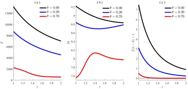
¹⁰

Panel (a) of Fig. 2 shows the responses of Y (τ, θ) to trade liberalization in a baseline case (θ = 0), a case with the lower level of labor market frictions (θ = 0.20), and a case with the higher level of labor market frictions (θ = 0.70).

Panel (b) does the same for U (τ, θ). Panel (c) illustrates whether the condition for saddle- path stability Γ(1 − δ) − 1 > 0 is met. (See the Appendix A for details.) As we can see, higher θ makes it more difficult to satisfy the stability condition. Thus, when we examine panels (a) and (b), we must focus on an area where Γ(1 − δ) > 1 is satisfied.

Figure 2: The impact of trade liberalization on GDP (a), welfare (b), and dynamic stability (c).

In panel (a), we find that trade liberalization leads to increases in GDP for θ ∈ [0, 0.20, 0.70].

In light of (28), this means that the sum of the first term and the third dominates the second for assumed parameter values. The main point here is that higher θ considerably weakens the beneficial impact of trade liberalization; for example, in the baseline case of θ = 0, moving from τ = 2 to τ = 1 has a huge impact on GDP. But when θ = 0.70, it has a much smaller effect. Therefore, policymakers must recognize that the impact of trade liberalization on economic growth is quite limited when the level of labor market frictions is high.

At the same time, it can be a strong policy tool to spur on economic growth when labor markets are frictionless (θ = 0) .

9

We can relax the assumption of f

X

= f

D

= f by, for example, choosing f

X

= 3.01 as in Felbermayr et al. (2011). That option, however, makes it difficult to interpret the numerical results since (28) and (29) are derived under that assumption. Moreover, our qualitative results remain unchanged even if we allow f

X

to be higher than f

D

. Thus, we continue to assume f

X

= f

D

= f to facilitate our exposition.

10

This should not be viewed as a formal calibration that can be compared quantitatively to facts about a

particular economy; the point is to show qualitatively what the responses of Y (τ, θ) and U (τ, θ) look like.

(15)

Next, Panel (b) shows the responses of U (τ, θ) to trade liberalization for θ ∈ [0, 0.20, 0.70].

In a frictionless limit (θ = 0), it delivers a welfare gain. When θ is low (θ = 0.20), we see a U-shaped relation; trade liberalization in a less open economy deteriorates welfare, while in a sufficiently open economy, it delivers a welfare gain. The initial reduction in U (τ, θ) is due to the second term in (29); when θ is low and a household anticipates higher dividend, trade liberalization encourages it to save more and consume less. Above a threshold, this effect being relatively mitigated, trade liberalization induces a household to consume more, thereby generating a U-shaped pattern. Thus, in this scenario, a less open economy cannot jointly raise long-run growth and welfare.

Finally, when θ is high (θ = 0.70), we see an inverted U-shaped relation; trade liberalization in a less open economy improves welfare, while in a sufficiently open economy, it delivers a welfare loss. This is again due to a household’s intertemporal optimal choice: when θ is high and a household anticipates lower dividend, the effect of the second term in (29) is little and trade liberalization encourages it to consume more. Above a threshold, this effect being relatively magnified, a household consumes less in response to trade liberalization, thereby generating an inverted U-shaped pattern. As such, when θ is high, a more open economy fail to jointly raise long-run growth and welfare.

The findings of this section can be summarized as follows:

Proposition 3. For assumed parameter values, regardless of the level of labor market frictions, trade liberalization leads to increases in GDP. When their level is lower, it delivers a welfare loss for a less open economy, and a welfare gain for a sufficiently open economy. In contrast, when their level is higher, it delivers a welfare gain for a less open economy, and a welfare loss for a sufficiently open economy.

5. Concluding Remarks

Can trade liberalization jointly raise long-run growth and welfare? To answer this question, we have developed a tractable dynamic trade model with firm heterogeneity and fair wages. In sharp contrast to standard Melitz (2003) models with endogenous growth, we do not assume ad hoc knowledge spillover. Defining GDP that is consistent with official statistics, we study the impact of trade liberalization on economic growth and welfare. In the baseline case where labor market frictions are in isolation, we have analytically shown that trade liberalization may lead to lower growth due to three forces and deliver a welfare loss due to four forces.

We then simulate our model to demonstrate that there is a critical interaction between

economic growth, welfare, openness, and the level of labor market frictions. For example,

in a less open economy with the lower level of labor market frictions, trade liberalization

delivers a welfare loss. This is also the case in a more open economy with the higher level of

labor market frictions. Therefore, the answer to our question critically hinges on the degree

of openness and how frictional labor markets are.

(16)

Acknowledgements

We thank participants at 63rd KMSG Seminar and 8th TLM Research Meeting for helpful comments. This work was supported by Grants-in-Aid for Scientific Research [KAKENHI:

18K01616]. The authors have no conflicts of interest to disclose.

Appendix A. Steady State and Stability Analysis

In this Appendix, we derive key steady state solutions and discuss the dynamic stability of our model by constructing a phase diagram. First, using Eqs. (15), (18), (19), and (26), we get the following dynamic relation:

M

_D,t+1

= (1 − δ)

1 + Λ

f

_e

(ZM

_D,t

)

^k

M

_D,t

− 1 − δ

f

_e

(ZM

_D,t

)

^k

C

_t

, (A.1) where Λ ≡ q − f

_D

[1 + nχ(f

_X

/f

_D

)]. To find loci, let us define the changes in the mass of producing firms ∆M

_D,t

≡ M

_D,t+1

− M

_D,t

. Substituting (A.1) into ∆M

_D,t

and rearranging, we have

∆M

_D,t

R 0 ⇔ C

_t

Q ΛM

_D,t

− f

_e

Z

^k

δ

1 − δ

M

_D,t^1+k

. (A.2) Next, inserting (14) and (20) into (23), using (19) and (18), and defining the changes in consumption ∆C

_t

≡ C

_t+1

− C

_t

, we find

∆C

t

R 0 ⇔ M

D,t+1

Γ(1 − δ) − (ZM

_D,t

)

^k

1 − δ

R M

D,t

1 − (ZM

D,t

)

^k

,

where Γ ≡ βf

_e⁻¹

(¯ π + f

_e

). For our purpose, it is useful to calculate the threshold value M

_D

as follows:

Γ(1 − δ) − (ZM

D,t

)

^k

> 0 ⇔ M

D,t

< [Γ(1 − δ)]

¹^k

Z ≡ M

_D

. We then have

∆C

_t

R 0 ⇔ M

_D,t+1

R (1 − δ)

1 − (ZM

_D,t

)

^k

Γ(1 − δ) − (ZM

_D,t

)

^k

M

_D,t

, for M

_D,t

∈ (0, M

_D

),

∆C

_t

R 0 ⇔ M

_D,t+1

Q (1 − δ)

1 − (ZM

_D,t

)

^k

Γ(1 − δ) − (ZM

_D,t

)

^k

M

_D,t

, for M

_D

< M

_D,t

. Inserting (A.1) into these, they become

∆C

_t

R 0 ⇔ C

_t

Q ΛM

_D,t

+ f

_e

Z

^k

M

_D,t^k+1

Γ(1 − δ) − 1 Γ(1 − δ) − (ZM

_D,t

)

^k

, for M

_D,t

∈ (0, M

_D

),

∆C

_t

R 0 ⇔ C

_t

R ΛM

_D,t

+ f

_e

Z

^k

M

_D,t^k+1

Γ(1 − δ) − 1 Γ(1 − δ) − (ZM

_D,t

)

^k

, for M

_D

< M

_D,t

.

(17)

Therefore, at the intersection of the ∆M

_D,t

= 0 locus and the ∆C

_t

= 0 locus, we can derive their steady-state values:

M

_D

= Z

⁻¹

(1 − δ)(Γ − 1) δ

¹_k

, C = Z

⁻¹

(1 − δ)(Γ − 1) δ

_k¹

[Λ − f

_e

(Γ − 1)] . (A.3) where we assume (1 − δ)(Γ − 1) > 0 ⇔ Γ > 1 for M

_D

> 0 and Λ − f

_e

(Γ − 1) > 0 for C > 0. Putting above information on steady state dynamics together, we can construct phase diagrams as shown in Figs. A.3 and A.4. Fig. A.3 considers the case where Γ(1 − δ) > 1. In this case, M

_D,t

and C

_t

move along the saddle path toward their steady-state values, hence establishing saddle-path stability. In contrast, when Γ(1 − δ) < 1, we can see an unstable spiral out away from the steady state. Therefore, in this case, the steady state is globally unstable. Given lim

θ→1

Γ(1 − δ) = β(1 − δ) < 1, the steady state tends to be globally unstable as the level of labor market frictions gets higher. As such, if not a sole parameter, θ strictly governs the dynamic stability of our model.

We complete this Appendix by providing the steady-state solution for Y : Y = qM

_D

= qZ

⁻¹

(1 − δ)(Γ − 1) δ

_k¹

. (A.4)

Those for the rest are obvious and thus omitted.

Figure A.3: The saddle-path stable case.

(18)

Figure A.4: The globally unstable case.

References

[1] Acemoglu, D., Ventura, J., 2002. The World Income Distribution. Quarterly Journal of Economics.

117(2), 659-694. https://doi.org/10.1162/003355302753650355

[2] Aghion, P., Howitt, P., 1994. Growth and Unemployment. Review of Economic Studies. 61(3), 477-494.

https://doi.org/10.2307/2297900

[3] Akerlof, G.A., Yellen, J.L., 1990. The Fair Wage-Effort Hypothesis and Unemployment. Quarterly Journal of Economics. 105(2), 255-283. https://doi.org/10.2307/2937787

[4] Baldwin, R.E., Robert-Nicoud, F., 2008. Trade and Growth with Heterogeneous Firms. Journal of International Economics. 74(1), 21-34. https://doi.org/10.1016/j.jinteco.2007.05.004

[5] Bernard, A.B., Redding, S.J., Schott, P.K., 2007. Comarative Advantage and Heterogeneous Firms.

Review of Economic Studies 74(1), 31-66. https://doi.org/10.1111/j.1467-937X.2007.00413.x [6] Blanchard, O., Giavazzi, F., 2003. Macroeconomic Effects of Regulation and Deregulation in Goods

and Labor Markets. Quarterly Journal of Economics. 118(3), 879-907. https://doi.org/10.1162/

00335530360698450

[7] Egger, H., Kreickemeier, U., 2009. Firm Heterogeneity and the Labor Market Effects of Trade Liber- alization. International Economic Review. 50(1), 187-216. https://doi.org/10.1111/j.1468-2354.

2008.00527.x

[8] Felbermayr, G., Prat, J., Schmerer, H-J., 2011. Globalization and Labor Market Outcomes: Wage Bargaining, Search Frictions, and Firm Heterogeneity. Journal of Economic Theory. 146(1), 39-73.

https://doi.org/10.1016/j.jet.2010.07.004

[9] Fukuda, K., 2019. Effects of Trade Liberalization on Growth and Welfare through Basic and Applied Researches. Journal of Macroeconomics. 62, 103058. https://doi.org/10.1016/j.jmacro.2018.08.

011 [10] Ghironi, F., Melitz, M.J., 2005. International Trade and Macroeconomic Dynamics with Heterogeneous

Firms. Quarterly Journal of Economics. 120(3), 865-915. https://doi.org/10.1093/qje/120.3.865

(19)

[11] Grossman, G.M., Helpman, E., 1991. Innovation and Growth in the Global Economy. Cambridge, Massachusetts: MIT Press.

[12] Gustafsson, P., Segerstrom, P., 2010. Trade Liberalization and Productivity Growth. Review of Inter- national Economics. 18(2), 207-228. https://doi.org/10.1111/j.1467-9396.2010.00878.x

[13] Melitz, M.J., 2003. The Impact of Trade on Intra-Industry Reallocations and Aggregate Industry Productivity. Econometrica. 71(6), 1695-1725. https://doi.org/10.1111/1468-0262.00467

[14] Naito, T., 2017. Growth and Welfare Effects of Unilateral Trade Liberalization with Heterogeneous Firms and Asymmetric Countries. Journal of International Economics. 109, 167-173. https://doi.

org/10.1016/j.jinteco.2017.08.011

[15] Ourens, G., 2016. Trade and Growth with Heterogeneous Firms Revisited. Journal of International Economics. 100, 194-202. https://doi.org/10.1016/j.jinteco.2016.03.006

[16] Ourens, G., 2020. The Long-term Impact of Trade with Firm Heterogeneity. Review of World Eco- nomics. (forthcoming) https://doi.org/10.1007/s10290-020-00384-0

[17] Rivera-Batiz, L.A., Romer, P.M., 1991a. International Trade with Endogenous Technological Change.

European Economic Review. 35(4), 971-1001. https://doi.org/10.1016/0014-2921(91)90048-N [18] Rivera-Batiz, L.A., Romer, P.M., 1991b. Economic Integration and Endogenous Growth. Quarterly

Journal of Economics. 106(2), 531-555. https://doi.org/10.2307/2937946

[19] Schubert, S.F., Turnovsky, S.J., 2018. Growth and Unemployment: Short-run and Long-run Tradeoffs.

Journal of Economic Dynamics and Control 91, 172-189. https://doi.org/10.1016/j.jedc.2017.

11.003 [20] Stepanok, I., 2018. A North-South Model of Trade with Search Unemployment. European Economic Review. 101, 546-566. https://doi.org/10.1016/j.euroecorev.2017.10.023

[21] Unel, B., 2010. Technology Diffusion through Trade with Heterogeneous Firms. Review of International Economics. 18(3), 465-481. https://doi.org/10.1111/j.1467-9396.2010.00880.x

[22] Unel, B., 2013. The Interaction between Technology Adoption and Trade When Firms Are Heteroge- neous. Review of International Economics. 21(4), 797-808. https://doi.org/10.1111/roie.12071 [23] Ventura, J., 2005. A Global View of Economic Growth. Handbook of Economic Growth. Vol. 1B,

Chapter 22, 1419-1497. https://doi.org/10.1016/S1574-0684(05)01022-1

[24] Wu, T.T., 2015. Firm Heterogeneity, Trade, Multinationals, and Growth: A Quantitative Evaluation.

Journal of International Economics. 97(2), 359-375. https://doi.org/10.1016/j.jinteco.2015.07.

004