Cavity-enhanced magnetometer with a spinor Bose Einstein condensate

Cavity‑enhanced magnetometer with a spinor Bose Einstein condensate

Author Karol Gietka, Farokh Mivehvar, Thomas Busch journal or

publication title

New Journal of Physics

volume 23

number 4

page range 043020

year 2021‑04‑08

Publisher IOP Publishing Ltd on behalf of the Institute of Physics and Deutsche Physikalische

Gesellschaft.

Rights (C) 2021 The Author(s). 

Author's flag publisher

URL http://id.nii.ac.jp/1394/00001911/

doi: info:doi/10.1088/1367-2630/abedff

Creative Commons Attribution 4.0 International(https://creativecommons.org/licenses/by/4.0/)

PAPER • OPEN ACCESS

Cavity-enhanced magnetometer with a spinor Bose–Einstein condensate

To cite this article: Karol Gietka et al 2021 New J. Phys. 23 043020

View the article online for updates and enhancements.

This content was downloaded from IP address 203.181.243.17 on 07/05/2021 at 02:16

New J. Phys.23(2021) 043020 https://doi.org/10.1088/1367-2630/abedff

O P E N AC C E S S

R E C E I V E D

18 November 2020

R E V I S E D

12 February 2021

AC C E P T E D F O R P U B L I C AT I O N

11 March 2021

P U B L I S H E D

8 April 2021

Original content from this work may be used under the terms of the Creative Commons Attribution 4.0 licence.

Any further distribution of this work must maintain attribution to the author(s) and the title of the work, journal citation and DOI.

PAPER

Cavity-enhanced magnetometer with a spinor Bose–Einstein condensate

Karol Gietka^1,∗ , Farokh Mivehvar² and Thomas Busch¹

1 Quantum Systems Unit, Okinawa Institute of Science and Technology Graduate University, Onna, Okinawa 904-0495, Japan

2 Institut für Theoretische Physik, Universit¨at Innsbruck, A-6020 Innsbruck, Austria

∗ Author to whom any correspondence should be addressed.

E-mail:[email protected]

Keywords:magnetometry, quantum metrology, spinor Bose–Einstein condensate, cavity QED, superradiance

Abstract

We propose a novel type of composite light–matter magnetometer based on a transversely driven multi-component Bose–Einstein condensate coupled to two distinct electromagnetic modes of a linear cavity. Above the critical pump strength, the change of the population imbalance of the condensate caused by an external magnetic field entails the change of relative photon number of the two cavity modes. Monitoring the cavity output fields thus allows for nondestructive measurement of the magnetic field in real time and we show that the sensitivity of the proposed magnetometer exhibits Heisenberg-like scaling with respect to the atom number. For

state-of-the-art experimental parameters, we calculate the lower bound on the sensitivity of such a system to be of the order of fT ( √

Hz)

⁻¹

–pT ( √

Hz)

⁻¹

for a condensate of 10

⁴

atoms with coherence times on the order of several ms.

1. Introduction

Being able to measure the direction, strength, and temporospatial dependence of magnetic fields with high accuracy has applications in various scientific fields, ranging from physics [1,

2] and geology [3] to biology

and medicine [4,

5]. High-precision magnetometers can be used to test fundamental physical theories [6–9]

and explore the boundaries of quantum metrology [10–14]. Until very recently, the progress in magnetometry was driven by superconducting quantum interference devices, which are based on superconducting loops containing Josephson junctions [15]. However, the technological developments in cooling, trapping, and manipulating ultracold atoms have led to the development of a next generation of atomic magnetometers [16–27]. Among them, Faraday-rotation magnetometers [28] have attracted a great deal of interest, as due to the possibility of increased noise suppression by creating non-classical states of light and atoms, they can operate on the verge or even beyond the standard quantum limit [29,

30]. Using

anti-relaxation coatings [20,

31], optical multi-pass cells [24], and, finally, spin-exchange relaxation-free

protocols [16,

17] has enabled to reach sensitivities as low as 160 aT (√

Hz)

⁻¹

[32]. Other state-of-the-art magnetometers rely on magnetostrictive optomechanical cavities, which can reach a peak magnetic field sensitivity of 400 nT (

√

Hz)

⁻¹

[33], and nitrogen-vacancy centers in diamonds [34–41], which can exhibit sensitivities up to the order of fT (

√

Hz)

⁻¹

.

In this work, we propose an alternative approach to measure magnetic field strengths based on light–matter interactions in an optical cavity [42–44]. In contrast to free space, where the back-action of the particles onto the trapping laser light is negligible, in optical cavities the optical dipole force on the atoms together with the atomic back-action onto the light field give rise to complex nonlinear coupled dynamics. Motivated by recent progress in strongly coupling ultracold atoms to high-Q optical cavities [45–54], we propose to harness these light–matter interactions as a sensitive probe for magnetic fields [55,

56]. The considered setup consists of a one-dimensional spinor (i.e. two-component) Bose–Einstein

condensate (BEC) in an external (static or time-dependent) magnetic field, transversely driven by two pump lasers and dispersively coupled to two distinct electromagnetic modes of a linear cavity as depicted in

© 2021 The Author(s). Published by IOP Publishing Ltd on behalf of the Institute of Physics and Deutsche Physikalische Gesellschaft

Figure 1. Schematic of the system. The atoms are strongly confined along the axis of an optical cavity and driven by two off-resonant transverse lasers with Rabi frequenciesΩ_jinducing internal atomic transitions|g_j ↔ |e_j. These transitions are also strongly coupled to two distinct standing-wave cavity modesˆajwith coupling strengthGj. The atoms can experience a Zeeman shift due to a static magnetic fieldBand/or a time-dependent magnetic fieldB_⊥cos(ωt), with the latter inducing transitions

|g₁ ↔ |g₂.

figure

1

[57,

58]. The relative occupation of the cavity modes depends on the state of the condensate, which

in turn is affected by the presence of the external magnetic field. Measuring the cavity-output fields, which can be done non-destructively, then allows for real-time and continuous measurements of the magnetic field. We find that the lower bound on the sensitivity of measuring the magnetic field is on the order of fT (

√

Hz)

⁻¹

–pT (

√

Hz)

⁻¹

for typical state-of-the-art experimental parameters. Although we consider this physical setting in the context of magnetometry, it can be easily extended to measurements of any field or force that can couple the spinor components of the BEC, as well as real-time monitoring of the population imbalance of a spinor condensate.

2. Model

The condensate we consider consists of N four-level atoms with mass M trapped along the axis of a two-mode standing-wave linear cavity by a tightly confining potential along the transverse directions. The atoms have two hyperfine ground states which are coherently driven from the transverse direction by two off-resonant external pump lasers, as depicted in figure

1, which induce transitions|

g

_j ↔ |

e

j

(j = 1, 2) with the Rabi frequency Ω

j

. The transition

|g_j ↔ |ej

is also coupled to a cavity mode ˆ a

j

with the mode function cos(k

_cj

x) and coupling strength

Gj

(x) =

Gj

cos(k

_cj

x), where

Gj

is the maximum single

atom-photon coupling rate. The pump and cavity frequencies, respectively, ω

p_j

and ω

c_j

= ck

c_j

= 2πc/λ

c_j

are assumed to be near resonant with each other, but far-red detuned with respect to the atomic frequencies ω

j

. The relative energy between the two lowest lying states can be changed with a static magnetic field B

that induces the Zeeman energy difference

γB

, where γ is the gyromagnetic ratio. These states can also be coupled with an ac magnetic field B

_⊥

cos ωt, introducing an (ac Zeeman) energy shift

ω, and inducing

magnetic dipole transition between

|

g

₁

and

|

g

₂

with a magnetic Raman frequency Ω = γB

_⊥

.

In the dispersive regime

|

Δ

_j| ≡ |

ω

_pj−

ω

_j| {

Ω

_j

;

Gj}

, in which the atomic excited states

|

e

_j

quickly reach a steady state, their dynamics can be adiabatically eliminated (see appendix

A). As a result, in the

rotating frame of the pumping lasers, the effective Hamiltonian for the atoms in the ground states and the cavity fields becomes

H ˆ =

Ψ ˆ

^†

(x)

H

ˆ

0

Ψ(x) dx ˆ

−Δc1

ˆ a

^†₁

ˆ a

1−Δc2

ˆ a

^†₂

ˆ a

2

, (2.1) where Ψ = ˆ ( ψ ˆ

1

, ψ ˆ

2

)

is the bosonic spinor field annihilation operator and

H

ˆ

0

is the single-particle

Hamiltonian density

H

ˆ

0

=

⎛

⎜⎝

ˆ p

²

2M + ˆ V

₁

(x)

−

γB

−

ω i Ω/2

−iΩ/2

ˆ p

²

2M + ˆ V

2

(x) +

δ

⎞

⎟⎠

. (2.2)

Here, V ˆ

j

(x) =

Uj

ˆ a

^†_j

ˆ a

j

cos

²

(k

c_j

x) +

ηj

(ˆ a

j

+ ˆ a

^†_j

) cos(k

c_j

x) is the dynamical cavity potential with

U

_j

=

G_j²

/Δ

j

being the maximum depth of the optical potential per photon due to the absorption and emission of cavity photons. The maximum depth of the optical potentials due to the redistribution of photons between the pump lasers and the cavity fields are given by

ηj

=

Gj

Ω

j

/Δ

j

, and δ = Ω

²₂

/Δ

2

−

Ω

²₁

/Δ

1

+ ω

12

is the Stark-shifted two-photon detuning, with ω

12

being the bare energy difference

New J. Phys.23(2021) 043020 K Gietkaet al

between

|

g

₁

and

|

g

₂

. For the sake of clarity, in remainder of this work we will focus on the balanced condition, i.e. U

0≡

U

1

= U

2

, Δ

c≡

Δ

c₁

= Δ

c₂

, ω

c ≡

ω

c₁

= ω

c₂

, k

c≡

k

c₁

= k

c₂

, and η

₀≡

η

₁

= η

₂

. We assume that the atom–atom interactions are negligible with respect to the cavity-mediated interactions, which is quantitatively a good approximation for spinor-BEC–cavity-quantum-electrodynamics experiments [49,

52].

In the mean-field approximation, the system is the described by a set of four coupled equations for the cavity-field amplitudes

ˆ a

_j

(t )

= α

j

(t ) and the atomic condensate wave functions

ψj

(x, t)

= ψ

_j

(x, t), given by

i ∂

∂t α

j

=

−Δc

+ U

0cos²

(k

c

x)

j−

iκ

α

j

+ η

0cos (kc

x)

j

, i ∂

∂t ψ

1

=

p

²

2M + V

1

(x)

−(γB

+ ω)

ψ

1

+ i Ω 2 ψ

2

, i ∂

∂t ψ

2

=

p

²

2M + V

2

(x) +

δ

ψ

2−

i Ω

2 ψ

1

, (2.3)

where V

j

(x) =

V ˆ

j

(x), and

cos²

(k

c

x)

j

and

cos(kc

x)

j

are spatial overlaps of cos

²

(k

c

x) and cos(k

c

x) with the corresponding atomic density

|ψj

(x)|

²

, respectively. Here we have introduced the cavity-photon loss rate κ which signifies the open nature of the system and is a crucial component in the model [51]. It provides a way for the system to reach a steady state and allows for non-destructive monitoring of this state.

It can be shown that this system can also be described by two coupled Dicke models [59], whose two low-lying polaritons are coupled by an external field [60,

61]. Since the effective spin formed by these two

polaritons is not coupled to the cavity field (no optical

|g₁ ↔ |g₂

transition), the only mechanism leading to the relaxation of the effective spin will be spontaneous emission, allowing for long coherence times and consequently long measurement times [62].

3. Magnetometry

We first consider a Ramsey scheme, for which we have

{

Ω, ω

}

= 0 [63]. The condensate is initially prepared in an equal superposition state (δN

≡

N

1−

N

2

= 0 with N

j

=

|ψ_j

(x, t)|

²

dx), and we subsequently turn on the static magnetic field B

which induces a Zeeman splitting

γB

of the energy levels. In this static magnetic field the two spinor components acquire a relative phase φ = τ γB

,

³

where τ is the interrogation time. After switching off the static magnetic field, a π/2 pulse is applied which converts the relative phase into a relative atom number. This can be easily seen if we introduce total pseudo-spin operators defined as ˆ

s

= Ψ ˆ

^†

σ Ψ ˆ dr, where σ is the vector of Pauli matrices. In particular, ˆ s

_z

= N

₁−

N

₂

= δN corresponds to the population imbalance. Any unitary transformation of such a pseudo-spin can be depicted as a rotation exp(−iφˆ s

n

/2) on the generalized Bloch sphere, where

n

and φ are the rotation axis and rotation angle, respectively. Introducing a pseudo-spin state

|

ϑ, ϕ

≡√

N

e

^iϕ

cos(ϑ/2)

|

g

₁

+ sin(ϑ/2)

|

g

₂

= Ψ ˆ dx, where ϑ and ϕ are the azimuthal and polar angles, the conversion of the relative phase to the relative atom number (

ϑ,

ϕ|ˆ s

_z|ϑ,

ϕ = N cos ϑ) can be conveniently expressed by e

^−iˆsxπ/4|π/2,

φ =

|π/2−

φ, 0. We note that in the superradiant regime where the strength of the effective cavity pump η

₀

is above a certain threshold, and which is the regime we focus on here, the average number of photons

|αj|²

in cavity mode j is proportional to the atom number N

j

in pseudo-spin state j; cf equation (2.3). By measuring the relative photon number

|

α

₁

(φ)

|²− |

α

₂

(φ)

|²≡

δn during or after a time interval t, one can then estimate the relative atom number δN and thus φ and the strength of the static magnetic field.

To measure an oscillating magnetic field B

_⊥

cos ωt, one can employ a Rabi scheme [64]. In the rotating frame of the oscillating magnetic field and in the presence of a small bias field, B

(fixing the axis of quantization), the relative energy between the two ground states is shifted by an amount

ω. The oscillating

field induces Rabi oscillations between the two components of the BEC with a frequency Ω = γB

_⊥

(see equation (2.2)), and for the resonant case

−γB−

ω = δ, the spinor components will oscillate without acquiring any relative phase. In this case the entire information about the amplitude of the magnetic field B

_⊥

is encoded in the period of the spinor oscillations, i.e. the oscillations of the relative number of atoms.

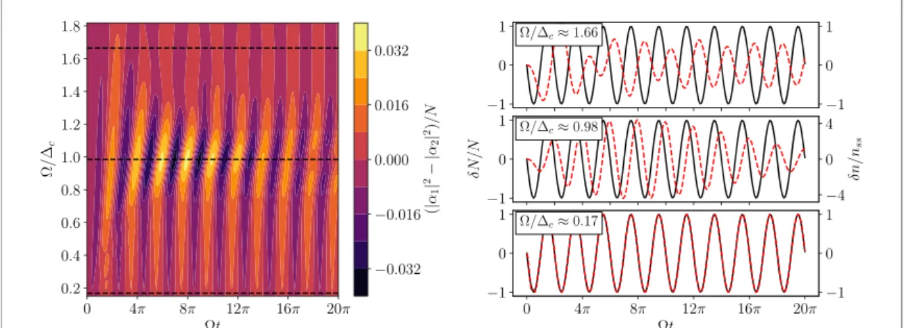
Since the photon scattering probability depends on the number of atoms, the spinor oscillations directly lead to oscillations of the cavity mode amplitudes with frequency Ω as well. In figure

2

we show the normalized relative photon number (|α

1|²− |α2|²

)/N as a function of (unitless) time Ωt and (unitless) frequency Ω/Δ

c

. In this graph one can clearly distinguish three distinct regimes of photon scattering. When

3For clarity, we have moved to the reference frame rotating with frequencyδ, so the accumulated phase is notφ=τ(γB+δ), but φ=τ γB.

3

Figure 2. Left-hand side: the normalized relative photon number (|α1|²− |α2|²)/Nas a function of the magnetic Rabi frequency Ωscaled by the cavity detuningΔcand timetnormalized to the Rabi frequencyΩ. An increasing shift between the oscillations of the spinor BEC and the relative average number of photons can be clearly seen: depending on the relative strength ofΩandΔc, one can identify three distinct photon-dynamics regions forΩ<|Δ_c|,Ω∼ |Δ_c|, andΩ>|Δ_c|(indicated by horizontal-black- dashed lines). Examples of these are presented on the right-hand side, where the solid-black line represents the normalized BEC population-imbalance oscillations and the dashed-red line represents the relative photon number oscillations normalized to the maximal number of scattered photons in the steady staten_ss(see equation (5.9)). The dashed-black lines on the left panel indicate the cuts presented on the right-hand side. See the text for detailed explanation. The parameters are set to (Δ_c,U₀,η₀,κ)=(−3300,−1/600, 300, 300)ω_randN=10⁴.

Ω <

|Δc|

, the optical potential adiabatically follows the atomic density oscillations. For Ω

∼ |Δc|

, the photon dynamics cannot completely follow the BEC population-imbalance oscillations, introducing a time delay between the BEC population-imbalance and cavity field-amplitude oscillations. Surprisingly, the number of scattered photons increases in this regime, leading to enhanced sensitivity with respect to the adiabatic case. Finally, when Ω >

|Δc|, the photon scattering cannot keep up with the Rabi oscillations of

the condensate, introducing thus a constant π phase shift between atomic and photonic oscillations. Hence, the number of scattered photons decreases until the relative atom number oscillations are so fast that they no longer affect scattering of photons (see appendix

B

for the details).

4. Measurement back-action

Even though our system allows for non-destructive measurement, an inevitable consequence of any measurement is the measurement back-action. This generally adds noise to the system and thus to the measurement outcomes themselves, which reduces the estimation precision [65]. In general, the

measurement-back action is a stochastic process and, in the limit of continuous measurement, the evolution of the system state ρ ˆ is governed by the stochastic master equation [66]

d ρ ˆ =

−

i

H, ˆ ρ ˆ

dt +

D

[ ˆ c]ˆ ρ dt +

√

H[ˆ c]ˆ ρ dW. (4.1)

Here we have defined the Lindblad superoperator

D[ˆ

c] := ˆ c ρˆ ˆ c

^†−

1

2

ˆ c

^†

ˆ c ρ ˆ + ˆ ρ ˆ c

^†

ˆ c

, (4.2)

the measurement superoperator

H[ˆ

c] := ˆ c ρ ˆ + ˆ ρˆ c

^†− ˆ

c + ˆ c

^†ˆ

ρ, (4.3) the Wiener process increment dW, and a measurement efficiency 1. The Lindblad superoperator describes the disturbance of the system due to the measurement, and the measurement superoperator represents the gain of information resulting from a measurement. For an arbitrary operator O, we can ˆ combine the stochastic master equation and d

O ˆ

= Tr[ O, dˆ ˆ ρ] to obtain the equation of motion for the expectation value of O ˆ as

d O ˆ =

−

i

O, ˆ H ˆ

dt +

ˆ c

^†

Oˆ ˆ c

−

1

2

ˆ

c

^†

ˆ c O ˆ + ˆ Oˆ c

^†

ˆ c

dt +

√

ˆ c

^†

O ˆ + ˆ Oˆ c

−

O ˆ ˆ c

^†

+ ˆ c

dW. (4.4)

New J. Phys.23(2021) 043020 K Gietkaet al

Figure 3. The effect of continuous measurement back-action on the cavity-field dynamics. Here we set the measurement efficiency equal to 50% (=0.5). Although the measurement back-action strongly affects single quantum trajectories (right), by averaging over many independent trajectories (for the calculations we used 100 trajectories) the noise averages out (left); cf figure2. The parameters for this simulation are the same as in figure2.

For a homodyne detection scheme, which can be used to measure the average number of photons [67], we have ˆ c =

√

2κˆ a, and if we set the measurement efficiency equal to zero, it is straightforward to re-derive equation (2.3). Since the atomic field operators ψ ˆ

j

commute with the cavity field operators ˆ a

j

, a non-zero measurement efficiency modifies the mean-field equations for the cavity fields as

i ∂

∂t α

j

=

−Δc

+ U

0cos²

(k

c

x)

j

α

j

+ η

0cos (kc

x)

j−

iκα

j

+ i

√

2κξ(t), (4.5)

where ξ(t) is white noise. In other words, in the mean-field limit the measurement back-action adds a stochastic noise to the cavity fields. This in turn leads to the deformation of the optical potentials inside the cavity and eventually to heating and loss of atoms. In the case of the Ramsey scheme, this can be

counteracted by a feedback loop [53] or included in the process of calibration. In the case of the Rabi scheme, the effect of the measurement back-action should be more pronounced as the number of scattered photons is a function of time. In order to obtain the average relative photon number, one would therefore have to repeat the experiment many times. Because the fluctuations of the optical potentials do not change the relative number of atoms in the condensate, our scheme realizes a non-demolition quantum

measurement of condensate state. This can be seen in figure

3, where we have plotted the averaged and

single quantum trajectories for different noise realizations of the relative average number of photons as a function of Ω for = 0.5.

5. Cavity-field measurement and sensitivity

After carrying out the full Ramsey scheme and reaching a stationary state, the relative average number of photons δn is measured for a time interval t and the value of the magnetic field B

is estimated from the collected data gathered by performing enough measurements to average out the effect of noise. The relative average number of detected photons during t will be

δn(φ) = κt

|α0|²

cos φ, (5.1) where

|α0|²

is the maximum number of scattered photons in a single mode. Subsequently, the value of φ is estimated with the sensitivity given by the error propagation formula

Δφ = Δ [δn(φ)]

∂

φ

[δn(φ)] = Δ|α

1

(φ)|

²

+ Δ|α

2

(φ)|

²

κt|α

0|²|

sin φ| . (5.2)

For classical fields, the uncertainty of the relative average number of photons can easily be estimated as Δ [δn(φ)]

≈√

κt

|α0|

, and the sensitivity for measuring B

becomes ΔB

= 1

γτ

√

κt

|

α

₀

sin φ

|

1 γτ

√

κt

|

α

₀|

. (5.3)

In the Rabi scheme case, even though the qualitative behavior of cavity fields is different in each regime of parameters (see appendix

B), the relative average number of photons inside the cavity oscillates with

5

frequency Ω as illustrated in figure

2. Therefore, measuring the cavity output fields should allow for

nondestructive measurement of Ω. We assume that the cavity field is detected over short time intervals δt during which the cavity output field is approximately constant and the measurement is repeated enough times to smooth out the fluctuations of the field. Then the instantaneous relative average number of detected photons at time t is

δn(t)

≈

κ

_t+δt/2

t−δt/2 |α0|²

cos Ωt

dt

≈

κδt|α

0|²

sin Ωt. (5.4)

Again, by comparing the measured data with the model in equation (5.4), the value of the magnetic field B

_⊥

can be estimated with the uncertainty given by the error propagation formula

ΔB

_⊥≈

1 γt

√

κδt

|

α

₀

sin(Ωt)

|

1 γt

√

κδt

|

α

₀|

. (5.5)

It is also instructive to refer to the quantum theory of estimation and calculate the quantum Fisher information, F

q

, which sets a lower bound on the sensitivity through the quantum Cram´ er–Rao bound as ΔB 1/

F

q

[68,

69]. For pure states the Fisher information is defined as

F

q

= 4(Δˆ h) with ˆ h = i[∂

BU

ˆ ]

U

ˆ

^†

being the generator of an infinitesimal change along a trajectory parametrized by B. From the viewpoint of the relative average number of cavity photons ˆ a = (ˆ a

1−

ˆ a

2

)/2 and in the reference frame in which α

1

, α

2∈R,⁴

the dynamics will be governed by the displacement operator

U

ˆ (t) = ˆ D(α) = exp

αˆ a

^†−

α

^∗

ˆ a

, (5.6)

where α = α

^∗≡

α(t) depends on the regime of photon scattering. The generator of the infinitesimal change ˆ h can be easily calculated as

ˆ h = i ∂α

∂B

ˆ a

^†−

ˆ a

, (5.7)

and from this the quantum Fisher information can be directly determined to be given by F

q

= 4(Δˆ h)

²

=

∂α

∂B

2

. (5.8)

It is easy to show that for both, the Ramsey scheme [α

≈ |α0|√

κt cos

γB

τ

] and the Rabi scheme [α

≈ |α0|√

κδt cos(γB

_⊥

t)], the quantum Cram´ er–Rao bound yields the same limitation on the sensitivity as equations (5.3) and (5.5).

Finally, let us make a comment concerning the average number of photons. The average number of cavity photons can be calculated using the steady-state solution. Deep in the self-ordered (superradiant) regime [70], we get

n

ss≡ |α0|²≈

N

²

η

²

[Δ

c−

NU

0

]

²

+ κ

²

, (5.9)

where Δ

c−

NU

0

is the dispersively shifted cavity detuning. Therefore, for negligible dispersive shift Δ

_c−

NU

₀≈

Δ

_c

, the average number of photons will be

|

α

₀|²∼

N

²

η

²

/(Δ

²_c

+ κ

²

), and from the viewpoint of the atoms, we obtain a Heisenberg-like scaling of the sensitivity similarly to what was found in [71]. In two-mode systems with a fixed number of particles, for example a collection of N interacting two-level atoms, the Heisenberg scaling means that the sensitivity scales like

∼

1/N. In the systems composed of solely atoms this can only be achieved with the use of entanglement. The achieved

∼

1/N scaling in our proposal, however, has its origins not in entanglement but in superradiance, which is a consequence of strong light–matter interaction. The information about the magnetic field is encoded linearly into the state of the atoms which are not entangled. Performing thus an optimal measurement directly on such atoms would give rise maximally to the standard quantum limit

∼

1/

√

N. That said, due to the strong coupling of the atoms to the cavity modes, the information about the magnetic field is also effectively imprinted into the state of the cavity fields. Since the average number of photons in the superradiant regime is

proportional to the number of atoms squared n

ss ∼

N

²

, measuring the cavity fields gives rise to a 1/N scaling of the sensitivity. Because the origin of this scaling is not entanglement, we call it Heisenberg-like scaling.

It is worth noting that since in the non-superradiant regime no photons is scattered into the cavity modes, the presented scheme requires to operate in the superradiant phase.

4We move to such a frame of reference for the clarity of calculations.

New J. Phys.23(2021) 043020 K Gietkaet al

6. Implementation and estimated sensitivity

This magnetometer proposal is based on existing experimental technologies for quantum-gas-cavity systems [48,

49,51–53]. For instance, the spinor BEC could be realized by coupling two internal states of⁸⁷

Rb,

|

F, m

_f

=

|

1,

−

1

≡ |↓

and

|

F, m

_f

=

|

2,

−

2

≡ |↑

to the cavity modes, similarly as in references [49,

52],

or by making use of the F = 1 total angular momentum manifold of a

⁸⁷

Rb by preparing the gas in the mixture of m

f

= +1 and m

f

=

−1 sub-levels as in reference [48]. Coupling the spins to two different cavity

modes could be realized by using two orthogonal polarizations [50] or two modes with different

frequencies [72]. We, therefore, attempt in the following to estimate the sensitivity lower bound by using state-of-the-art experimental parameters from recent spinor-BEC-cavity experiments [48,

51]. Assuming

that one performs m = T/t

s

experiments with T being the total time of the experiment and t

s

being the time of a single experiment which may consist of many measurements, for Ramsey scheme we obtain

ΔB

√

T =

√

t

s

γτ

√

κt

|α0|

, (6.1)

and for Rabi scheme we find

ΔB

_⊥√

T =

√

t

_s

γt

√

κδt

|α0|

. (6.2)

Assuming

⁸⁷

Rb atoms with a gyromagnetic ratio of γ = 2π

×

7 Hz nT

⁻¹

, an experimental cycle time of the order of 1 s, a coherence time of the order of 10 ms, and ideal photon detectors, the lower bound on the sensitivity of the cavity-based magnetometer containing around 10

^{4 87}

Rb atoms would be

ΔB

√

T

∼

fT (

√

Hz)

⁻¹

for a Ramsey scheme and ΔB

_⊥√

T

∼

10 pT (

√

Hz)

⁻¹

for the Rabi scheme.

However, under realistic conditions, i.e. taking into account experimental and measurement back-action noise, limitations associated with heating the condensate by strong intra-cavity lattices [53], and dispersion of the cavity deforming the interference lattice, a realistic sensitivity will be much lower. Taking the average number of photons from [52] the sensitivity of the proposed magnetometer would rather be on the order of

∼

10 pT(

√

Hz)

⁻¹

for the Ramsey scheme and

∼

100 nT(

√

Hz)

⁻¹

for the Rabi scheme, which is comparable with other state-of-the-art magnetometers. The proposed magnetometer should be also possible to be implemented in ensembles of thermal atoms which realize two coupled Dicke systems [50,

55,56].

In principle, one can also loosen the balanced condition, and consider a limiting case where one measures only a single mode of the cavity, ˆ a

j

. In this case the intra-cavity field amplitude will behave as

|αj| ≈|α0|

2 [1

±

cos(φ)] . (6.3)

Inserting this expression into the formula for the quantum Fisher information (5.8), it is straightforward to show that the lower bound of the sensitivity will be two times higher than the bounds from equations (5.3) and (5.5).

7. Outlook and conclusions

We have presented an experimentally realistic scheme for the highly-precise measurement of a magnetic field strength based on light–matter interaction inside a two-mode linear cavity. On the one hand, the back-action of the atoms onto the light fields transfers the information about the coupling to the cavity field, and on the other hand, the cavity fields help to trap the atoms in many lattice sites. Importantly this also allows to non-destructively monitor the dynamics of the system. Since the proposed magnetometer operates in the superradiant regime, it, therefore, exhibits a Heisenberg-like scaling of the sensitivity.

We have found that the lower bound on the sensitivity of such a magnetometer is on the order of

∼

fT (

√

Hz)

⁻¹

for a Ramsey scheme and

∼

10 pT (

√

Hz)

⁻¹

for the Rabi scheme, assuming total

measurement times on the order of 1 s and condensates with about 10

⁴

atoms. The concept of the proposed magnetometer is built upon the fact that a change of the relative occupation of the spinor components leads to a change of the relative average number of photons which can be measured through the cavity-output fields. Although we have shown how to exploit the light–matter interaction for magnetometry, the scope of this physical setting can be easily extended to measure any type of field or force that can modify or couple spinor components of the BEC. From a different perspective, the proposed setup allows to monitor the state and dynamics of a spinor BEC in real time. An interesting extension would be to additionally take

advantage of light–matter interaction to create non-classical states of matter and/or light and further increase the sensitivity of the proposed machine [10,

73–76]. One can easily imagine that number squeezing

of the cavity fields would reduce the sensitivity below the photon shot-noise limit. Unfortunately, a full

7

quantum treatment of such a system would require gargantuan computational power and, except for few body problems and semi-classical models, it is currently beyond the scope of theoretical investigations [77].

Acknowledgments

Simulations were performed using the open-source QuantumOptics.jl framework in Julia [78]. KG would like to acknowledge discussions with Stefan Ostermann, David Plankensteiner, Helmut Ritsch, Juan Polo Gomez, James Kwiecinski, Jan Kołody´ nski and also correspondence with Tobias Donner and Ronen Kroeze.

This work was supported by the Okinawa Institute of Science and Technology Graduate University. KG acknowledges support from the Japanese Society for the Promotion of Science (P19792). FM is supported by the Lise-Meitner Fellowship M2438-NBL of the Austrian Science Fund (FWF), and the International Joint Project No. I3964-N27 of the FWF and the National Agency for Research (ANR) of France.

Data availability statement

The data that support the findings of this study are available upon reasonable request from the authors.

Appendix A. Effective model

The energies of the states of the four-level bosonic atoms are

ωg1

=

−γB

,

ωg2

,

ωe1

, and

ωe2

(see the main text for details). In the dipole and the rotating wave approximations, the single-particle Hamiltonian density becomes

H

ˆ = ˆ p

²

2M I

_4×4

+

ξ={g1,g₂,e₁,e₂}

ωξ

σ ˆ

ξξ

+

ωc1

ˆ a

^†₁

ˆ a

1

+

ωc2

ˆ a

^†₂

ˆ a

2

+

G1

(x)ˆ a

1

ˆ σ

e1g1

+

G2

(x)ˆ a

2

σ ˆ

e2g2

+ H.c.

+ Ω

1

e

^−iωp1t

ˆ σ

e1g1

+ Ω

2

e

^−iωp2t

σ ˆ

e2g2

+ H.c.

+ Ω e

^−iωt

σ ˆ

g1g2

+ H.c.

,

(A.1)

where m is the atomic mass, ˆ a

j

is the annihilation operator of cavity photons in cavity mode j, ˆ

σ

ξξ ≡ |ξξ|,

ˆ p is the center-of-mass momentum operator of the atom along the cavity axis x, I

_4×4

is the identity matrix in the internal atomic-state space, and H.c. stands for the Hermitian conjugate. In the rotating frame of the pumping lasers,

H

˜ =

UHU^†

+ i

_∂

∂tU

U^†

, using the unitary transformation

U

= exp

i

−ωp₁−

ω

p₂

+ ω 2

ˆ σ

g₁g₁

+

−ωp₁−

ω

p₂−

ω 2

ˆ σ

g₂g₂

+

ω

_p1−

ω

_p2

+ ω 2

ˆ σ

e1e1

+

−

ω

_p1

+ ω

_p2−

ω 2

ˆ

σ

e2e2

+ ω

p₁

ˆ a

^†₁

ˆ a

₁

+ ω

p₂

ˆ a

^†₂

ˆ a

₂

t

,

(A.2)

the single-particle Hamiltonian density becomes

H

˜ = ˆ p

²

2M I

_4×4

+

Δg1

σ ˆ

g1g1

+

Δg2

σ ˆ

g2g2−Δe1

σ ˆ

e1e1−Δe2

σ ˆ

e2e2−Δc₁

ˆ a

^†₁

ˆ a

−Δc2

ˆ a

^†₂

ˆ a

2

+

G1

(x)ˆ a

1

σ ˆ

e1g1

+

G2

(x)ˆ a

2

σ ˆ

e2g2

+ H.c.

+ Ω

1

σ ˆ

e1g1

+ Ω

2

σ ˆ

e2g2

+ H.c.

+ Ωˆ σ

g1g2

+ H.c.

,

(A.3)

where we have defined Δ

_g1 ≡

ω

_g1

+ (ω

_p1

+ ω

_p2−

ω)/2, Δ

_g2 ≡

ω

_g2

+ (ω

_p1

+ ω

_p2

+ ω)/2, Δ

_e1 ≡ −

ω

_e1

+ (ω

p₁−

ω

p₂

+ ω)/2, Δ

e₂ ≡ −ωe₂

+ (ω

p₁

+ ω

p₂−

ω)/2, and Δ

c_j ≡

ω

p_j−

ω

c_j

as the atomic and cavity detunings with respect to the pump lasers and oscillating magnetic field. The many-body Hamiltonian is

H ˆ =

Ψ ˆ

^†

(x)

M

˜ Ψ(x) dx, ˆ (A.4)

where Ψ(x) ˆ = ( ψ ˆ

g1

, ψ ˆ

g2

, ψ ˆ

e1

, ψ ˆ

e2

)

are the bosonic field operators satisfying

ψ ˆ

ξ

(x), ψ ˆ

^†_ξ

(x

)

= δ

ξ,ξ

δ(x

−

x

),

and

M

˜ is the matrix form of the Hamiltonian density

H

˜ . Using this many-body Hamiltonian, we can write

New J. Phys.23(2021) 043020 K Gietkaet al

the Heisenberg equations of motion of the photonic and atomic field operators i ∂

∂t ˆ a

j

=

−Δc_j

ˆ a

j−

iκˆ a

j

+

Gj

(x) ψ ˆ

^†_gj

ψ ˆ

ej

dx, (A.5) i ∂

∂t ψ ˆ

_g1

= p

²

2M + Δ

_g1

ψ ˆ

_g1

+

G1

(x)ˆ a

^†₁

+ Ω

₁

ψ ˆ

_e1

+ Ω ˆ ψ

_g2

, (A.6)

i ∂

∂t ψ ˆ

g₂

= p

²

2M +

Δg₂

ψ ˆ

g₂

+

G2

(x)ˆ a

^†₂

+ Ω

2

ψ ˆ

e₂

+

Ω ˆ

ψ

g₁

, (A.7)

i ∂

∂t ψ ˆ

e_j

= p

²

2M

−Δe_j

ψ ˆ

e_j

+

Gj

(x)ˆ a

j

+ Ω

j

ψ ˆ

g_j

, (A.8)

where

−

iκˆ a

_j

corresponds to the decay of the cavity mode j. In the limit of large atomic detunings Δ

ej

, the atomic field operators

{

ψ ˆ

e1

, ψ ˆ

e2}

of the excited states reach quickly steady states, allowing for adiabatic elimination of their dynamics. Assuming the kinetic energies are negligible with respect to

−Δe1

and

−Δe2

, we obtain the steady-state solutions for the atomic field operators of the excited states as

ψ ˆ

ej

= 1 Δ

ej

Gj

(x)ˆ a

_j

+ Ω

j

ψ ˆ

gj

. (A.9)

If we now insert the above steady-state solutions into the Heisenberg equations of motion (A.5), we obtain effective equations for the photonic and atomic field operators

i ∂

∂t ˆ a

_j

=

−

Δ

_cj−

iκ + U

_j

ψ ˆ

^†_j

cos

²

(k

_cj

x) ψ ˆ

_j

dx

ˆ a

_j

+ η

_j

ψ ˆ

^†_j

cos(k

_cj

x) ψ ˆ

_j

dx, (A.10) i ∂

∂t ψ ˆ

1

= p

²

2M

−γB−ω

+

U1

cos

²

(k

c₁

x) +

η1

cos(k

c₁

x)

ˆ a

1

+ ˆ a

^†₁

ψ ˆ

1

+

Ω ˆ

ψ

2

, (A.11)

i ∂

∂t ψ ˆ

2

= p

²

2M +

δ

+

U2

cos

²

(k

c₂

x) +

η2

cos(k

c₂

x)

ˆ a

1

+ ˆ a

^†₁

ψ

2

+

Ω ˆ

ψ

1

, (A.12) where ψ ˆ

_j≡

ψ ˆ

_gj

, Δ

_j≡

Δ

_ej

, U

_j≡ Gj²

/Δ

_j

, η

_j≡ Gj

Ω

_j

/Δ

_j

, and δ = Ω

²₂

/Δ

₂−

Ω

²₁

/Δ

₁

+ ω

_g2

. Finally, using the mean-field approximation and replacing the photonic and atomic field operators ˆ a

_j

and ψ ˆ

gj

with their corresponding averages α

j≡ ˆ

a

j

and ψ ˆ

g_j ≡

ψ

g_j

, respectively yields the following equations of motion

i ∂

∂t α

j

=

−Δc

+ U

0cos²

(k

c

x)

j−

iκ

α

j

+ η

0cos (kc

x)

j

, (A.13) i ∂

∂t ψ

1

=

p

²

2M + V

1

(x)

−(γB

+ ω)

ψ

1

+ i Ω

2 ψ

2

, (A.14)

i ∂

∂t ψ

2

=

p

²

2M + V

₂

(x) +

δ

ψ

2−

i Ω

2 ψ

1

. (A.15)

Appendix B. Cavity fields

The equations that govern the dynamics of cavity fields are given by (for clarity of the calculations, we have assumed the balanced condition, i.e. U

1

= U

2≡

U

0

, Δ

c1

= Δ

c2 ≡

Δ

c

, ω

c1

= ω

c2

= ω

c

, and η

₁

= η

₂≡

η

₀

)

i ∂

∂t α

j

=

−Δc

+ U

0cos²

(k

c

x)

j−

iκ

α

j

+ η

0cos (kc

x)

j

. (B.1) Assuming that we are deep in the self-ordered regime, the two integrals for spinor component j = 1 read

cos (kc

x)

1

= cos

²

(φ/2)

ψ ˆ

^†₁

(x) cos(k

c

x) ψ ˆ

1

(x)dx =

−N

cos

²

(φ/2), (B.2)

cos

²

(k

_c

x)

1

= cos

²

(φ/2)

ψ ˆ

^†₁

(x)cos

²

(k

_c

x) ψ ˆ

1

(x)dx = N cos

²

(φ/2), (B.3) and for j = 2

cos (k

_c

x)

2

= sin

²

(φ/2)

ψ ˆ

^†₂

(x) cos(k

_c

x) ψ ˆ

2

(x)dx =

−

N sin

²

(φ/2), (B.4)

9