Astudy on Order Statistics from Nonidentically Distributed Kumaraswamy Variables
Z. AL-Saiary
Department of Statistics, College of Science, King Abdulaziz University [email protected]
Abstract: In this work I dedused the moments of order statistics of independent nonidentically (inid) distributed Kumaraswamy random variables. Numerical calculations for different values of the parameters from this distribution are given. I computed the first two moments and the variance of the second order statistics of sample size n = 3. The last order statistics of sample size n = 2 in the presence of multiple outliers are obtained. All calculations are tabulated. Graphs of pdf, cdf for the rth (inid) order statistics are found.
[Z. AL-Saiary. Astudy on Order Statistics from Nonidentically Distributed Kumaraswamy Variables. Academ Arena 2016;8(10):27-32]. ISSN 1553-992X (print); ISSN 2158-771X (online). http://www.sciencepub.net/academia.
2. doi:10.7537/marsaaj081016.02.
Key words: Order statistics, Moments, non-identically distributed, Kumaraswamy distribution.
Introduction
There are three trends have emerged in the literature to obtain moments of order statistics of (inid) distributed random variables. One of these trends is initiated by (Balakrishnan, 1994). He exploited the known relation between the probability density function (pdf) and the cumulative distribution function (cdf). Other trend using survival function, this trend establish by Barakat and Abdelkader (2003). Last trend was established by Jamjoom and Alsaiary (2011). In this last trend researchers using the moment
generating functiontechnique. In this paper we computed the moments of OS arising from INID distributed Kumaraswamy random variables using second The study of OS from INID rvs is started in the
literature by (Vaughan and Venables, 1972; David, 1981; Bapat and Beg, 1989; David and Nagaraja, 2003). (Balakrishnan, 1994) derived recurrence relations for single and product moments of OS from INID rvs for the Exponential distribution. Childs and Balakrishnan (2006) derived the moments of OS from
INID rvs for Logistic distribution. (Mohamed et al., 2007) else applied Balakrishnan method for doubly truncated Lomax, Weibull-Gamma, Burr XII and for general class of distributions. The second trend was applied by (Barakat and Abdelkader, 2000) in weibull distribution and then they generalized this method in (2003) and used it in Erlang distribution. Jamjoom and AL-Saiary (2012) applied it to beta type I with three parameters random variables. The survival function of Gamma and Beta distributions used by Abdelkader (2004) and (Abdelkader, 2008) to compute the moments of OS from INID rvs for beta distribution.
AL-Saiary (2015) applied the third trend to Standard type II Generalized logistic random variables.
Kumaraswamy Distribution
The probability density function of a random variable X from Kumaraswamy distribution is given by:
a 1 a b 1
a b x 1 x , a 0 , b 0 , 0 x 1 f (x)
0, otherwise
The cumulative distribution function is given as:
a b
F(x) 1 1 x , a 0 , b 0 , 0 x 1
a and b are shape parameters. See Kumaraswamy (1980).
Nonidentical Order Statistics from Kumaraswamy Distribution:
Let , , …, be independent random variables having cumulative distribution functions ( ), ( ), … , ( ) and probability density functions ( ), ( ), … , ( ), respectively. Let : ≤ : ≤…
: denote the order statistics obtained by arranging the n , in increasing order of magnitude. Then the p.d.f and the c.d.f of the rth order statistic : (1≤ ≤ ≤) can be written as:
Where p
denotes the summation over all n! permutations ( , ,…, ) (1, 2, … ). (Bapat and Beg, 1989) put it in the form of permanent as:
1 1
( ) 1 ( ) ( ) 1 ( ) ( 3)
: ! ( , 1)
r n r
fr n x n r n r per F x f x F x
( ) ( ) 1 ( ) ( 4 )
( ) 1 1
j n
F x n F x F x
r j r pj a i a a j ia
pj
is all permutations of i i1, 2,,in
for (1,, )n which satisify i1i2ij and
1 2
j j n
i i i
. And using permanent as:
1( ) 1 1( )
( ) 1 , (5)
( ) ( 1)! ( 1, 1)
( ) 1 ( )
n
i r
n n
i n i
F x F x
F x per x
r n i n i
F x F x
we can obtain the p.d.f. and the c.d.f. of the first INID OS of KW distribution when n = 3 from eq (1) and (2) IN ( 3 ) AND ( 4 ) using (Permanent) and Mathematica Program as:
3
( ) 1 1 1 , 0, 0, 0 ( 7 )
1:3
a bi
F x x i x a bi
Figure 1: Graphs of p.d.f. and c.d.f of (inid) OS.from KW distribution for selected values of b2 = 1, b3 = 2, b1= 1, 2, 3,4, 5, n = 5, a = 0.5
Moments of OS from INID Kumaraswamy rvs:
Now, we consider the case when the variables X1, X2,…,Xn be INID rvs having cdfs:
a bi
F(x) 1 1 x , a 0, b 0 , 0 x 1, i 1, 2,..., n
i
1
1 1
( ) 1 ( ) ( ) 1 ( ) ( 2 )
: ! ( , 1) a r c
r n
i i i
p a c r
f x F x f x F x
r n n r n r
3
3
( ) 1 1 1 , 0, 0, 0 ( 6 )
1: 3 1
a a bi
f x a b xi x i x a b
i
Now We will use theorem of (Barakat and Abdelkader, 2003) to deduse the moments of OS from INID rvs arising from our distribution.
Theorem 1: Let X1, X2,…,Xn be independent nonidentically distributed rvs. The kth moment of all order statistics,
(k)r:n
, for 1 r n and k = 1, 2,… is given by:
j (n r 1)
n j 1
(k) ( 1) I (k)
r:n j n r 1 n r j
(5)
Where:
k 1 j
I (k) ... k x G (x)dx, j 12,...,n
j 1 i i1 2 ij n 0 t 1 it
(6) Git (x) = 1- Fit (x) with (i1, i2,…, in) is a permutation of (1, 2,…, n ) for which i1i2<,…, <in.
The following theorem gives an explicit expression for Ij(k) when X1, X2,…, Xn are OS from INID Kumaraswamy rvs.
Theorem 2: For any real numbers a, b > 0, 1 r n and k = 1, 2,…
k j k
I (k) ... b 1,
j 1 i i ... i n a t 1 it a
1 2 j
(7) Proof: Applying theorem 1 and usingequation (4), we get:
j bi t 1 t
1 k 1 a
I (k) k ... x 1 x dx
j 1 i i i n 0
1 2 j
Substituting
y x a
the a above equation reduces to:
j t 1bit
1 k 1
k a
I (k) ... 1 y y dy
j 1 i i ... i n a 0
1 2 j
k j k
I (k) ... ( b 1, )
j 1 i i ... i n a t 1 it a
1 2 j
where, (a,b) is the beta function defined by:
1xa 1(1 x)b 1dx (a,b)
0
Remark 1: The kth moment of the last OS Xn:n from INID of Kumaraswamy rvs. can be written as:
(k) n ( 1)j 1I (k)
n:n j 1 j
(8)
where, Ij (k) is defined in (7)
Remark 2: The kth moment of the first OS X1:n from INID of Kumaraswamy rvs. can be written as:
(k) I (k)n
1:n
(9) Where:
k n k
I (k)n a i 1bi 1,a , a 0
(10)
Remark 3: For the Independent Identically Distributed (IID) case, we used betheorem 2. Ij(k) is be written as:
k n k
I (k) jb 1,
j a j a
(11)
Numerical calculations for Kumaraswamy distribution:
For k = 1, we dedused the following results:
Example 1
Let n = 3 and a =1, b1 = 1,, b2 = 2, b3 = (1(0.5) 4).. Table 1 shows the results.
Table 1: represents the first two moments and the variance of the median of inid OS when n = 3 and a =1, b1 = 1,, b2
= 2, b3 = (1(0.5) 4).
b3 1 1.5 2 2.5 3 3.5 4
E(x) 0.433333 0.3943 0.366667 0.346348 0.330952 0.318998 0.309524
E ( x )2 0.233333 0.195904 0.171429 0.154701 0.142857 0.134225 0.127778 V ( x ) 0.0455556 0.0404315 0.0369841 0.0347439 0.0333277 0.0324651 0.0319728
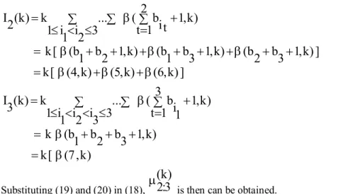
For example in (5) Let n = 3 and a =1, b 1, b 2 , b 3 1 2 3
. the kth moment of the median X2:3 is given by:
3 j 1
(k) ( 1)j 2 I (k)
2:3 j 2 1 j
I (k) 2I (k)
2 3
(18)
From (7):
I (k) k ... ( 2 b 1,k)
2 1 i i 3 t 1 it
1 2
k [ (b b 1,k) (b b 1,k) (b b 1,k) ]
1 2 1 3 2 3
k[ (4,k) (5,k) (6,k) ]
(19)
I (k) k ... ( 3 b 1,k)
3 1 i i1 2 3i 3 t 1 i1 k (b b b 1,k)
1 2 3
k[ (7 ,k)
(20) Substituting (19) and (20) in (18),
(k)
2:3
is then can be obtained.
Table 1 introduces the first two moments and the variance of the median from sample size
n = 3 arising from Kumaraswamy distribution. These computations are done when (a= 1, b1 = 1,, b2 = 2, b3 = (1(0.5) 4).
Example 2
Setting n = 2, a = 2, and b1 =1 (1) 5,b2 = 1 (1) 5, in Theorems 1 and 2, we get the following tables.
Table (2): The mean of the last inid OS of sample size n = 2 arising from Kumaraswamy distribution
b2
b1
1 2 3 4 5
1 0.8 0.742857 0.71746 0.703608 0.695083
2 0.742857 0.660317 0.621068 0.59869 0.584482
3 0.71746 0.621068 0.573293 0.545233 0.527013
4 0.703608 0.59869 0.545233 0.51316 0.491984
5 0.695083 0.584482 0.527013 0.491984 0.468557
For example, when k = 1, a = 2, b1 = 2, b2 = 3
I (1) I (1)
2:2 1 2
(23) From (7):
I (1) 2 ( b 1, )
1 i 1 i
[ (b 1, ) (b 1, ) ]
1 2
[ (3, ) (4, ) ]
1 1
2 2
1 1 1 1
2 2 2 2
1 1 1
2 2 2
(24) 1 2
I (1) ( b 1, )
2 2 t 1 1i
1 (b b 1,1 )
1 2
2 2
1 ( 6 , )1
2 2
1
2
(25)
Substituting (24) and (25) in (23), (k)
2:2
is then can be obtained.
Table (3): The second moment of the last inid OS of sample size n = 2 arising from Kumaraswamy distribution b2
b1
1 2 3 4 5
1 0.666667 0.583333 0.55 0.533333 0.52381
2 0.583333 0.466667 0.416667 0.390476 0.375
3 0.55 0.416667 0.357143 0.325 0.305556
4 0.533333 0.390476 0.325 0.288889 0.266667
5 0.52381 0.375 0.305556 0.266667 0.242424
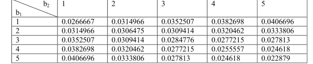
Table (4): The variance of the last inid OS of sample size n = 2 arising from Kumaraswamy distribution b2
b1
1 2 3 4 5
1 0.0266667 0.0314966 0.0352507 0.0382698 0.0406696
2 0.0314966 0.0306475 0.0309414 0.0320462 0.0333806
3 0.0352507 0.0309414 0.0284776 0.0277215 0.027813
4 0.0382698 0.0320462 0.0277215 0.0255557 0.024618
5 0.0406696 0.0333806 0.027813 0.024618 0.022879
Table 2 represents the mean of the last OS of sample size n = 2 arising from Kumaraswamy distribution.
These computations are done when ( n = 2, a = 1, and b1 =1 (1) 5,b2 = 1 (1) 5).
References
1. Abdelkader, Y., 2004. Computing the moments of order statistics from nonidentically distributed Gamma variables with applications. Int. J. Math.
Game Theo. Algebra., 14.
2. Abdelkader, Y., 2008. Computing the moments of order statistics from independent nonidentically distributed Beta random variables.
Stat. Pap., 49: 136-49.
3. Al-Saiary, Z., 2105. Order statistics from non- identical Standard type II Generalized logistic variables and applications at moments. American Journal of Theoretical and Applied Statistics.
4(1): 1-5.
4. Balakrishnan, N., 1994. Order statistics from non-identically exponential random variables and some applications. Comput. Stat. Data Anal., 18:
203-253.
5. Bapat, R.B. and M.I. BEG, 1989. Order statistics from non-identically distributed variables and permanents. Sankhya, A., 51: 79-93.
6. Barakat, H. and Y. Abdelkader, 2003. Computing the moments of order statistics from nonidentical random variables. Stat. Meth. Appl., 13: 15-26.
7. Barakat, H.M. and Y.H. Abdelkader, 2000.
Computing the moments of order statistics from nonidentically distributed Weibull variables. J.
Comp. Applied Math., 117: 85-90.
8. Childs, A. and N. Balakrishnan, 2006. Relations for order statistics from non-identical logistic random variables and assessment of the effect of multiple outliers on bias of linear estimators. J.
Stat. Plann. Inference., 136: 2227-2253.
9. David, H.A. and H.N. Nagaraja, 2003. Order Statistics. 3rd Edn., Wiley, New York.
10. David, H.A., 1981. Order Statistics. 2nd Edn., Wiley, New York.
11. Kumaraswamy, P., 1980. Generalized probability density-function for double- bounded random- processes, J. Hydrol. 46, pp. 79-88.
12. Mohmed, M., M. Mohie Elidin, M. Mahmoud and M. Moshref, 2007. On independent and nonidentical order statistics and associated inference. Department of Mathematics, (MSc.
Thesis) Cairo, AL-Azhar University.
13. Vaughan, R.J. and W.N. Venables, 1972.
Permanent expressions for order statistics densities. J. R. Statist. Soc., 34: 08-10.
10/15/2016


![I, §3] that the Schur functionsλ(x1](data:image/gif;base64,R0lGODlhAQABAIAAAP///wAAACH5BAEAAAAALAAAAAABAAEAAAICRAEAOw==)