A Semidefinite Programming Relaxation Approach for the Pooling Problem

A Semidefinite Programming Relaxation Approach for the Pooling Problem

Guidance

Associate Professor Nobuo YAMASHITA

Takahiro NISHI

Department of Applied Mathematics and Physics Graduate School of Informatics

Kyoto University

KYOTO UNIVER SIT

Y

F OU

ND E D 1897 KYOTO JAPAN

February 2010

A Semidefinite Programming Relaxation Approach for the Pooling Problem

Takahiro NISHI

Abstract

The pooling problem is to determine a scheduling of flows among several tanks in refinery processes of raw materials, such as crude oil and fuel gas. The refinery company first imports raw materials, and then produces final products by refining or mixing the materials in intermediate tanks, and finally send them to their consumers. The consumers require a certain level of quality of the final product. The pooling problem is regarded as a kind of the network flow problem.

However, it has two difficulties as compared to the usual linear network flow problem. One is an existence of pipeline constraints, which is formulated by using binary variables. The other is that the process of mixing materials are formulated as nonlinear equations. Thus, the pooling problem is a mixed-integer nonlinear programming. Moreover, even if the binary variables are fixed, the problem is nonconvex, and hence still very difficult. Therefore, we cannot apply the general-purpose solvers for the mixed-integer linear programming or the mixed-integer nonlinear programming.

In this paper, we apply semidefinite programming (SDP) relaxations for the polynomial optimization problem (POP) equivalent to the pooling problem. A solution of the SDP relaxation to the POP is known to be a reasonable solution. However, the size of the SDP tends to be very large and its solution is not necessarily feasible for the original POP. Therefore, we first propose a formulation of the pooling problem without the binary variables in order to reduce the problem size. Then, to tighten the relaxation, we consider to add some valid inequalities.

The valid inequality is a redundant constraint of the original problem. However, it may reduce the volume of the feasible region of the SDP, and hence we can expect to get a better solution.

Finally, in order to get a feasible solution of the original pooling problem, we formulate a

mixed-integer linear problem whose solution is feasible. Since the formulated problem includes

information of the solution of the SDP relaxation, its solution is expected to be a reasonable

feasible solution. We present some results of numerical experiments to show the validity of the

proposed approach.

Contents

1 Introduction 1

2 The Pooling Problem 3

3 Semidefinite Programming Relaxation Approach 8

3.1 Reformulation of the pooling problem to POP . . . . 8

3.2 Removal of u from (12) . . . . 9

3.3 Valid inequalities of (13) . . . . 10

3.4 Fixing variables after solving the SDP relaxation problem . . . . 12

3.5 Finding a feasible solution . . . . 13

3.6 Summary of the proposed approach . . . . 14

4 Numerical Experiments 15

5 Concluding Remarks 21

A Problem Data for Numerical Experiments 23

1 Introduction

The scheduling problem is one of the main problems in operations research, and arises in vari- ous fields, for example, resource allocation, job-shop scheduling, and process scheduling which includes batch processing, oil refinery and chemical processing. For some scheduling problems, efficient algorithms have been developed [3, 14]. In particular, problems formulated as the mixed integer problem (MIP) can be solved by the state-of-the-art MIP solvers. In this paper, we con- sider the pooling problem, which is one of the process scheduling problems formulated as the mixed-integer nonlinear problem.

The pooling problem is to determine a scheduling of flows among several tanks in refinery processes, such as crude oil and fuel gas [1, 2, 9]. A gas corporation or an oil company imports raw materials, produces final products by refining or mixing the materials, and send them to their consumers, such as industrial plants and households. A large amount of materials is imported at one time, and they usually have different qualities depending on their location of origin. The quality represents the value per unit amount, for example, a sulfur composition and an octane number for crude oil and a heating (calorific) value for fuel gas. The customers buy a small amount of the final product in a long period, and require a certain level of its quality.

If the requirement is not satisfied, then the company has to charge off the loss, such as costs for adding some expensive high quality materials in order to fill a deficit. Thus, the company puts the intermediate tanks where he stores materials temporarily and mixes materials to generate the final products. In this paper, we assume that there exist three types of components: the places where raw materials are imported (Source), the intermediate tanks which store materials temporarily and mix them (BlendTank), and customers who consume the final products are (Plant). In addition to these components, the problem has pipelines (Pipeline) which connect the components.

Since Sources, BlendTanks and Plants are regarded as nodes and Pipelines are regarded as edges, the pooling problem is to determine flows of materials in the network. Thus, the pooling problem can be regarded as a kind of network flow problem. However, it has two difficulties as compared to the usual linear network flow problems. The first difficulty appears in the constraints associated with Pipelines. When we use a pipeline, the amount of the material a that flows in the pipeline must be more than the lower capacity L and be less than the upper capacity U , i.e., L ≤ a ≤ U . On the other hand, when we do not use the pipeline, the amount of the material must be zero, which is inconsistent with L ≤ a. To overcome the inconsistency, we may employ the following binary variable which represents the use of the pipeline, i.e.,

u =

{ 1 (the pipeline is used) 0 (otherwise).

By using the binary variable, we can represent the constraints of flow a in the pipeline as follows:

uL ≤ a ≤ uU.

Each component, especially BlendTank, is connected with several pipelines. Those pipelines

cannot be used at the same time in order to prevent a back-flow and so on for safety. Thus we

use at most one pipeline in each time period. The requirement is represented by the constraints

that the sum of binary variables corresponding to the pipelines connected with the component

should not exceed one at each time. Second, the process of mixing materials are formulated

as nonlinear equations, and hence the pooling problem has nonlinear equality constraints. We explain the constraints. Consider two materials 1 and 2 to be mixed into the new material 3.

Suppose that the materials 1, 2 and 3 have the amounts p ₁ , p ₂ and p ₃ and qualities (which are values per unit amount) q 1 , q 2 and q 3 , respectively. Then, the following two equalities express proportional blending:

p 3 = p 1 + p 2

p 3 q 3 = p 1 q 1 + p 2 q 2 .

The first equation represents the mass balance and it is linear. The second equation means that the quality of the new material is calculated by the weighted average, and it is nonlinear.

Thus, the pooling problem can be written as a mixed-integer nonlinear programming problem.

Moreover, even if the binary variables are fixed, the problem is a nonconvex problem. Therefore, we cannot expect to compute a global optimal solution for practical scale pooling problems, and hence we consider to obtain a reasonable solution within practical time.

A lot of methods have been proposed to solve general mixed-integer nonlinear programming problems. For instance, the outer-approximation method [5] and the generalized Benders de- composition method [8] are well studied. Both methods can obtain a local optimal solution by solving continuous linear subproblems repeatedly if the problem obtained by fixing the integer part is convex. However, since the pooling problem is nonconvex as mentioned above, these method are not guaranteed to obtain a global optimal solution. Several methods tailored to the pooling problem have been proposed, including the combined method of graph theory and linear programming, and the genetic algorithm [4]. The former method first calculates a lower bound of the pooling problem by solving a continuous linear subproblem without some difficult constraints, and then obtains a feasible solution by solving a minimum cost flow problem. The latter one solves a combinatorial problem of the binary variables as an upper level problem, and continuous subproblems with the binary variables fixed are solved for each gene. Since both methods ignore nonlinear constraints to generate a trial point, they cannot well treat the nonlinear functions.

In this paper, we propose to apply the semidefinite programming relaxation for the pooling problem. As mentioned above, the pooling problem is formulated as a mixed-integer nonlinear problem. As shown in Section 3, the pooling problem can be written as a continuous polynomial optimization problem (POP). The POP is a nonlinear programming problem whose objective function and constraint functions are polynomial. Finding a global solution of POP is also difficult in general because a polynomial function might be nonconvex. In recent years, as a promising approach to solve the POP, the semidefinite programming relaxation has been attracted much attention [6, 11, 10, 13, 15]. A problem in which all the monomials included in the POP are linearized is formulated as a semidefinite programming problem (SDP), and it is a relaxation of the original POP. The SDP can be solved by the primal-dual interior point method. We can get its solution efficiently. In addition, Kojima et al. [7, 17] proposed a method to reduce the size of the SDP by using the sparsity of polynomials. As a result, an approximate solution is expected to be obtained within a reasonable computational time.

The main problem of applying the SDP relaxation is that the size of the SDP becomes very

large and the solution of the SDP is not necessarily feasible for the original problem. For example,

when we consider scheduling with 10 discrete time horizon, 10 components and 50 pipelines, the

pooling problem is formulated as a POP with 1200 variables, and its SDP relaxation problem

has at least a 1200×1200 matrix. In order to reduce the problem size, we propose a formulation that does not include the binary variables of the pooling problem. However, the removal causes excessive relaxation of the feasible region of the original problem. To tighten the region, we use valid inequalities. The valid inequality is known to be effective for the SDP relaxation approach.

It is a redundant constraint of the original POP, but it reduces the feasible region of the SDP, and hence we can expect to get a better solution. Moreover, we also consider to fix some of the variables after we solve the SDP relaxation problem. Then, we repeatedly solve the SDP relaxation problem with some variables fixed until we need not fix the variables. Finally, in order to get a feasible solution of the pooling problem, we propose to solve a mixed-integer linear programming problem by exploiting the information of the solution obtained by solving the final relaxation problem. The problem can be solved more easily than the original pooling problem.

The remainder of the present paper is organized as follows. Section 2 describes the formula- tion of the pooling problem. The semidefinite programming relaxation approach for the pooling problem is proposed in Section 3. Numerical results are presented and discussed in Section 4.

Finally, we make some concluding remarks in Section 5.

Throughout the paper, we use the following notations. For matrix X ∈ R ⁿ

ⁿ , X ≽ 0 means X is positive semidefinite, i.e., v ^T Xv ≥ 0 for all v ∈ R ⁿ . For x ∈ R ⁿ , ∥x∥ 1 = ∑ _n

i=1 |x i |. In addition, for a set A, | A | represents the number of elements in A.

2 The Pooling Problem

In this section, we give a concrete formulation of the pooling problem, and discuss its difficulties.

The purpose of the pooling problem is to determine schedules of flows of materials, from importing raw materials (e.g., crude oil and fuel gas) to sending final products to consumers.

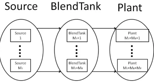
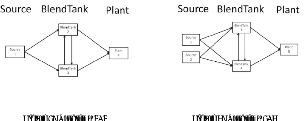
We consider a system that has three types of components, Source, BlendTank and Plant, and pipelines that connect the components. Source imports the raw materials at specific times.

BlendTank stores and blends (mixes) the materials, and generates the final products. Plant consumes (buys) the final products. The situation is shown in Fig.1.

Each material has its own quality. The quality is the value per unit amount, for example, an octane number of gasoline and a heating (calorific) value of fuel gas. Here, high quality implies good material. The raw materials imported to Source have a variety of quantity and quality. However, Plant requires a certain amount of quantity and a certain level of quality of the final products at each time. If that requirement is not satisfied, then the insufficiency of the requirement cause some additional cost. Therefore, intermediate tanks (BlendTank) are placed in the system for the reason not only to store the materials but also to mix them in order to satisfy the requirement of the quality. There are types of two costs in the pooling problem.

First, we transport the materials from one tank to another tank by electric power. This cost is called the “transportation cost”. Second, when the requirement of the quality is not satisfied, the company must pay extra money as mentioned above. We call this cost the “compensation cost”. We aim to minimize the sum of the total transportation costs and the total compensation costs.

The system in the pooling problem has a graph geometry where each component is regarded

as a node, and each pipeline as an edge. Here, we denote the numbers of Sources, BlendTanks,

Plants as M S , M B and M P , respectively. The number of all nodes M V is defined to be M V =

Figure 1: Overview of the pooling problem

M _S + M _B + M _P . Additionally, we denote the set of Sources by V _S , the set of BlendTanks by V B and the set of Plants by V P .

V _S = { 1, . . . , M _S } ,

V _B = { M _S + 1, . . . , M _S + M _B } ,

V _P = { M _S + M _B + 1, . . . , M _S + M _B + M _P } .

Let the set of all components be V . If there exists a pipeline that originates from node i and is destined for node j, we denote this pipeline as edge (i, j). The set of all edges is denoted as A. Here, we note that a pipeline has a direction, that is, we cannot transport from node j to node i by pipeline (i, j). For each node i ∈ V , we denote the set of nodes that have the edge destined for node i and the set of nodes that have the edge originating from node i by I (i) and E(i), respectively. Namely I(i) and E(i) are given as

I(i) ≡ { j ∈ V | (j, i) ∈ A } , E(i) ≡ { k ∈ V | (i, k) ∈ A } .

We formulate the problem with a uniform discretization of time in the given scheduling horizon. Let the final time of the horizon be M _T , and let the set of discretized times be T = { t | 1, . . . , M T } . In the following, we use indices i, j, and k for nodes and t for time period.

The notations for the graph and indexes are summarized in Table 1.

Next, we list given constants and decision variables of the pooling problem.

(a) Initial conditions for Source (constants)

Table 1: Notation of parameter of graph and indices Parameter of graph

M S : Cardinality of Source ． M _B : Cardinality of BlendTank ． M _P : Cardinality of Plant ． M V : The number of all nodes ．

M _T : The number of discretization of time horizon ． V _S : Set of Source ．

V B : Set of BlendTank ． V _P : Set of Plant ．

V : Set of all nodes ．

A: Set of all edges that represent pipeline ． I (i): Set of node which has an edge into node i ． E(i): Set of node which has an edge from node i ．

T : Set of discretized time ． Indices

i, j, k: Indices for each node.

t: Index for time period ． (i, j): Index for each edge ．

p ⁰ _i : Initial amount of materials in source i ∈ V _S ． q _i ⁰ : Initial quality of materials in source i ∈ V S ．

SA ^t _i : The amount of raw materials filled in source i ∈ V S at time t ∈ T ． SQ ^t _i : The quality of raw materials filled in source i ∈ V _S at time t ∈ T ． (b) Initial conditions for BlendTank (constants)

p ⁰ _i : Initial amount of materials in BlendTank i ∈ V _B ． q ⁰ _i : Initial quality of materials in BlendTank i ∈ V B ． p ^min _i : Minimum capacity of BlendTank i ∈ V _B ．

p ^max _i : Maximum capacity of BlendTank i ∈ V _B ． (c) Constants for Plant

DC _i ^t : The requirement of quantity in Plant i ∈ V P at time t ∈ T ． DQ ^t _i : The requirement of quality in Plant i ∈ V _P at time t ∈ T ．

CQ _i : Compensation cost per unit insufficiency of quality in Plant i ∈ V _P ． (d) Initial conditions for pipeline

L _ij : Lower bound on flow in edge (i, j) ． U ij : Upper bound on flow in edge (i, j) ． CA _ij : Cost per unit material flow of edge (i, j) ． (e) Decision variables for Source, BlendTank and Plant

p ^t _i : The amount of materials in node i ∈ V at time t ∈ T .

q _i ^t : The quality of materials in node i ∈ V at time t ∈ T .

(f) Decision variables for pipeline

a ^t _ij : The flow of edge (i, j) ∈ A at time t ∈ T .

u ^t _ij : binary variable indicating the usage of edge (i, j).

We denote the vector (p ¹ _i , . . . , p ^M _i

)

as p _i and the vector (p

, . . . , p

)

as p. Similarly, we denote other vector variables as q, a, u.

We formulate the pooling problem as a mixed-integer programming problem. The objective of this problem is to minimize the sum of transportation costs and compensation costs. The compensation cost is proportional to the product of the quality insufficiency and the amount of the final product. The concrete objective function of the problem can therefore be written as

∑

t

T

∑

(i,j)

A

CA _ij a _ij + ∑

t

T

∑

i

V

CQ _i DC _i ^t max { 0, DQ ^t _i − q _i ^t } . (1) We note that the compensation cost is higher than the transportation cost in general. If we need to satisfy the requirement of the quality, we set CQ := ∞ , which means that we add q _i ^t ≥ DQ ^t _i as constraints.

Next we describe the constraints. First, we note that when two materials are mixed, the newly generated material must have the same total amount and the same total value of the materials. As mentioned in Introduction, when we mix two materials 1 and 2 with quantity p 1 , p 2

and quality q ₁ , q ₂ into the new material 3 with quantity p ₃ and quality q ₃ , the following two equalities express proportional blending.

p ₃ = p ₁ + p ₂ (2)

p ₃ q ₃ = p ₁ q ₁ + p ₂ q ₂ (3)

The first equation (2) represents the material quantity balance, and it is linear. We call this equation the “quantity conservation law”. The second equation (3) represents the material quality balance, and it is nonlinear. This equation is called the “value conservation law”.

Now we give the whole constraints of the pooling problem.

Source constraints

The quantity conservation law (2) and the value conservation law (3) must be satisfied at all times, and the new raw material with the amount SA ^t _i and quality SQ ^t _i is added in time t ∈ T .

p ^t+1 _i = p ^t _i + SA ^t _i − ∑

k

E(i)

a ^t _ik ,

p ^t+1 _i q ^t+1 _i = p ^t _i q ^t _i + SA ^t _i SQ ^t _i − ∑

k

E(i)

a ^t _ik q ^t _i .

(4)

Additionally, the amount of material of each Source i ∈ V _S must be nonnegative at all times t ∈ T .

p ^t _i ≥ 0. (5)

BlendTank constraints

The quantity conservation law (2) and the value conservation law (3) must be satisfied at

all times.

p ^t+1 _i = p ^t _i + ∑

j

I(i)

a ^t _ji − ∑

k

E(i)

a ^t _ik ,

p ^t+1 _i q _i ^t+1 = p ^t _i q _i ^t + ∑

j

I(i)

a ^t _ji q _j ^t − ∑

k

E(i)

a ^t _ik q _i ^t .

(6)

A BlendTank i ∈ V B cannot be filled to more than its capacity and must keep the amount no less than its minimum volume.

p ^min _i ≤ p ^t _i ≤ p ^max _i . (7)

Plant constraints

In plant i ∈ V _P , the required amount of the final products is given by DC _i ^t in each time t ∈ T , and the total value is ∑

j

I(i) a ^t _ji q _j ^t . Thus the quality q ^t+1 _i is written as q _i ^t+1 =

∑

j

I(i) a ^t _ji q _j ^t

DC _i ^t . (8)

Pipeline constraints

For each pipeline (i, j) ∈ A, if there exists flow in time t ∈ T , we set binary variable u ^t _ij = 1, otherwise we set u ^t _ij = 0. Thus flow a ^t _ij must satisfy

u ^t _ij L _ij ≤ a ^t _ij ≤ u ^t _ij U _ij . (9) In each node i ∈ V , we can use at most one pipeline connected to node i. This requirement

can be formulated as ∑

j

I(i)

u ^t _ji + ∑

k

E(i)

u ^t _ik ≤ 1. (10)

Summarizing the above arguments from (1) to (10) ， we give the concrete pooling problem as follows.

(P) minimize

a,u,p,q

∑

t∈T

∑

(i,j)∈A

CA

a

+ ∑

t∈T

∑

i∈V_P

CQ

DC

max { 0, DQ

− q

}

subject to u

L

≤ a

≤ u

U

( ∀ (i, j) ∈ A, ∀ t ∈ T )

∑

j∈I(i)

u

+ ∑

k∈E(i)

u

≤ 1 ( ∀ i ∈ V, ∀ t ∈ T )

u

∈ { 0, 1 } ( ∀ (i, j) ∈ A, ∀ t ∈ T ) (a, p, q) ∈ Ω, ¯

(11)

where

Ω = ¯ { (a, p, q) | (4), (5), (6), (7), and (8) } .

Since the pooling problem has binary variables u = (u ^t _ij ), it is very difficult to solve. Another

difficult aspect is that it includes nonlinear functions in the constraints, i.e., the value conserva-

tion law (3). Since the value conservation law (3) is a nonlinear equation (not inequality), the

pooling problem cannot be a convex problem even if we fix the binary variables u. A mixed-

integer nonlinear programming problem can be solved by some algorithms, such as generalized

Benders decomposition method [8] and outer approximation method [5]. However, as mentioned

in Introduction, because they need the convexity of the subproblems obtained by fixing the in- teger part, they cannot be applied to the pooling problem. Moreover, even if we fix the binary variables, we cannot easily obtain a global solution, because many nonconvex constraints still remain. In addition to this difficulty, the number of binary variables is M T × |A|. When the scale of the problem becomes large, the combination of binary variables u grows exponentially.

Thus, it is difficult to apply the state-of-the-art method for combinational problems, such as Branch and Bound algorithms, to the pooling problem. Therefore, we must develop methods that are tailored to the pooling problem.

3 Semidefinite Programming Relaxation Approach

In this section, we propose a framework for solving the pooling problem (11) using the semidef- inite programming (SDP) relaxation approach. For applying the approach, we first reformulate the pooling problem as a polynomial optimization problem (POP). The POP is a nonlinear programming problem whose objective and constraint functions are polynomial. The standard form of POP is

(POP) minimize f ₀ (x)

subject to f _i (x) ≥ 0 (i = 1, . . . , m),

where all functions f _i : R ⁿ → R (i = 0, . . . , m) are polynomial. Note that equality constraints g(x) = 0 can be formulated as two inequalities of g(x) ≥ 0 and −g(x) ≥ 0 ．

By linearizing all monomials included in the POP, the POP is transfered into the linear SDP [11]. The SDP relaxation problem SDR _r (POP) of the POP can be written as

SDR r (POP) minimize F 0 (y)

subject to F _i (y) ≽ O (i = 1, . . . , m) M _r (y) ≽ O,

where r is the relaxation order, each F _i is a linearized function of f _i , and M _r is a symmetric matrix called a moment matrix (see [11] for details). The moment matrix M r plays an important role in the tightness of the relaxation, because it guarantees that a solution of the problem SDR _r (POP) coincides with a solution of the problem POP when relaxation order r is sufficiently large [11]. However, since the size of M r is n+r C r × n+r C r , the size of the problem SDR r (POP) increases exponentially as r and n, and hence it is very difficult to solve. Since the pooling problem (11) has at most quadratic functions, we can choose any relaxation order r ≥ 1. While the SDR 1 (POP) has an (n + 1) × (n + 1) matrix as its decision variables, and the SDR 2 (POP) has an ⁿ⁽ⁿ⁺¹⁾ ₂ × ⁿ⁽ⁿ⁺¹⁾ ₂ matrix. Thus when n = 100, the largest matrix size of SDR ₁ (POP) is 10, 201, while SDR 2 (POP) is 25, 502, 500. Since the pooling problem usually has hundreds of variables, we have to choose r = 1. However, note that a solution of the problem SDR r (POP) with lower r is not always feasible for the POP.

3.1 Reformulation of the pooling problem to POP

Here we give a POP formulation equivalent to the pooling problem (11). The pooling prob-

lem (11) includes max functions and binary valuables, and thus it is not a POP. First note that

u ^t _ij ∈ {0, 1} can be written as the polynomial constraint u ^t _ij (u ^t _ij −1) = 0, (∀ (i, j) ∈ A, ∀ t ∈ T ).

Thus, using the auxiliary variables v _i ^t (i ∈ V P , t ∈ T ) for the max functions, the pooling prob- lem (11) is written as

(P-POP) minimize

a,u,p,q,v

∑

t

T

∑

(i,j)

A

CA _ij a ^t _ij + ∑

t

T

∑

i

V

CQ _i DC _i ^t v _i ^t

subject to u ^t _ij L ij ≤ a ^t _ij ≤ u ^t _ij U ij (∀(i, j) ∈ A, ∀t ∈ T )

∑

j

I(i)

u ^t _ji + ∑

k

E(i)

u ^t _ik ≤ 1 ( ∀ i ∈ V, ∀ t ∈ T ) u ^t _ij (u ^t _ij − 1) = 0 (∀(i, j) ∈ A, ∀t ∈ T ) u ^t _ij ∈ R ( ∀ (i, j) ∈ A, ∀ t ∈ T ) (a, p, q, v) ∈ Ω,

(12)

where

Ω = { (a, p, q, v) | (a, p, q) ∈ Ω, v ¯ ^t _i ≥ DQ ^t _i − q _i ^t , v ^t _i ≥ 0 } .

We try to get an approximate solution of the problem (12) by the SDP relaxation approach.

We denote the SDP relaxation problem of the problem (12) with relaxation order r as SDR

r (P-POP) ． By solving the problem SDR r (P-POP), we can obtain an approximate solution (¯ a, u, ¯ p, ¯ q, ¯ v) of the original problem (12) ¯ ． If the approximate solution (¯ a, u, ¯ p, ¯ q, ¯ v) is feasible ¯ for the original problem (12), then (¯ a, u, ¯ p, ¯ q, ¯ v) is an optimal solution of the original prob- ¯ lem (12). However, the approximate solution (¯ a, u, ¯ p, ¯ q, ¯ v) is not necessarily feasible for the ¯ original problem (12) ． To obtain an optimal solution of (12), we must set the relaxation order r to be large enough. However, SDR r (P-POP) becomes huge for a large r. For example, consider a scheduling problem with 10 discrete time horizon, 10 components and 30 pipelines. Then the total number of variables is about 800, the size of the largest matrix in SDR ₁ (P-POP) is about 800 × 800, and the size of the largest matrix in SDR 2 (P-POP) is about 320, 000 × 320, 000.

Therefore, it is practically impossible to solve the SDP relaxation with relaxation order r ≥ 2.

We consider to obtain a reasonable approximate solution from SDR ₁ (P-POP).

Even if r = 1, the problem SDR 1 (P-POP) is still large. In Subsection 3.2, we first propose a formulation without u ^t _ij in order to reduce the problem size. The relaxation order r = 1 may imply that the relaxation is very loose. Thus, in Subsection 3.3, we consider to add appropriate valid inequalities to the problem in order to obtain a better approximate solution. In Subsection 3.4, we propose a procedure to fix some of flow variables a ^t _ij at zero after we solve the SDP relaxation problem, which reduces the size of the problem. The reduced SDP relaxation may provide a tight relaxation. Finally, in Subsection 3.5, in order to get a feasible solution of the original pooling problem, we formulate a mixed-integer linear programming problem whose solution is feasible for the pooling problem. Since the formulated problem includes information of the solution of the SDP relaxation problem, its solution is expected to be a reasonable feasible solution.

3.2 Removal of u from (12)

When we reduce the number of variables in (12), we can reduce the size of the SDP relaxation problem drastically, because the size of the SDP relaxation problem is usually the square of that of the original problem. Thus, we consider to remove u since they are artificial variables.

However, the deletion causes the following problem. We cannot represent the constraint (10)

that means we can use at most one pipeline connected to the same node at the same time, and the constraint (9) that represents for each pipeline (i, j) ∈ A, if flow exists in time t ∈ T, flow a ^t _ij satisfies L _ij ≤ a ^t _ij ≤ U _ij , otherwise a ^t _ij = 0.

To represent the constraint (10), we propose to add the following complementarity conditions.

a ^t _ji a ^t _ki = 0 (j, k ∈ I(i), j ̸ = k), a ^t _ij a ^t _ik = 0 (j, k ∈ E(i), j ̸ = k), a ^t _ji a ^t _ik = 0 (j ∈ I(i), k ∈ E(i)).

Moreover, since a ^t _ij ≥ 0 ( ∀ (i, j) ∈ A, ∀ t ∈ T ), these constraints are equal to following constraint.

∑

j,k

I(i),j

=k

a ^t _ji a ^t _ki + ∑

j,k

E(i),j

=k

a ^t _ij a ^t _ik + ∑

j

I(i),k

E(i)

a ^t _ji a ^t _ik = 0.

Next, to represent (9), we relax the constraint L ij ≤ a ^t _ij when flow exists. That is, we replace the constraint (9) by the following constraint.

0 ≤ a ^t _ij ≤ U _ij . Now we get the following relaxed problem of (12).

(P-POP) minimize

a,u,p,q,v

∑

t

T

∑

(i,j)

A

CA ij a ^t _ij + ∑

t

T

∑

i

V

CQ i DC _i ^t v _i ^t

subject to ∑

j,k

I(i),j

=k

a ^t _ji a ^t _ki + ∑

j,k

E(i),j

=k

a ^t _ij a ^t _ik + ∑

j

I(i),k

E(i)

a ^t _ji a ^t _ik = 0 (∀i ∈ V, ∀t ∈ T)

0 ≤ a ^t _ij ≤ U ij (∀(i, j) ∈ A, ∀t ∈ T )

(a, p, q, v) ∈ Ω.

(13) The number of variables of the problem (13) is M _T ×| A | fewer than those of the original problem (12). On the other hand, the number of the constraints of the problem (13) is the same as that of the original problem (12).

3.3 Valid inequalities of (13)

A valid inequality is known to be effective for the SDP relaxation approach. Although the valid inequality is a redundant constraint for the original POP, it tightens the feasible region of SDP, and hence we can expect to get a better solution. Especially, since the difficulty of the pooling problem comes from the value conservation law (3), it is effective to add valid inequalities related to the quality and pipeline constraints. We denote the problem (P-POP) with valid inequalities as (P-POP v ).

Trivial upper and lower bounds of each variable: Each variable has trivial upper and lower bounds. For example, the quality variable q ^t _i has an upper (lower) bound which is given by the largest (smallest) quality value of the given constants. Specifically, we set q ^max = max _i,t { q _i ⁰ , SQ ^t _i } and q ^min = min _i,t { q _i ⁰ , SQ ^t _i } . In this case, q ^t _i has the following valid inequalities.

q ^min ≤ q _i ^t ≤ q ^max . (14)

Note that it is time invariant. Since the quality of the final product must be greater than the worst case quality q ^min , the compensation variable v ^t _i must satisfy

v ^t _i ≤ DQ ^t _i − q ^min . (15)

Upper and lower bounds of monomials with degree 2: For monomial xy with 0 ≤ L x ≤ x ≤ U x

and 0 ≤ L y ≤ y ≤ U y ， the following inequalities hold [12].

xy ≤ U _y x + L _x y − L _x U _y , xy ≤ L _y x + U _x y − U _x L _y , xy ≥ U _y x + U _x y − U _x U _y , xy ≥ L _y x + L _x y − L _x L _y .

Using these relations, p ^min _i ≤ p ^t _i ≤ p ^max _i and q ^min ≤ q _i ^t ≤ q ^max give the following valid inequalities.

p ^t _i q ^t _i ≤ q ^max p ^t _i + p ^min _i q ^t _i − p ^min _i q ^max , p ^t _i q ^t _i ≤ q ^min p ^t _i + p ^max _i q ^t _i − p ^max _i q ^min , (16) p ^t _i q ^t _i ≥ q ^max p ^t _i + p ^max _i q _i ^t − p ^max _i q ^max , p ^t _i q ^t _i ≥ q ^min p ^t _i + p ^min _i q _i ^t − p ^min _i q ^min , (17) (q ^t _i ) ² ≤ (q ^min + q ^max )q _i ^t − q ^min q ^max , (18) (q ^t _i ) ² ≥ 2q ^max q ^t _i − (q ^max ) ² , (q _i ^t ) ² ≥ 2q ^min q ^t _i − (q ^min ) ² . (19) The monomials a ^t _ij q _i ^t , (p ^t _i ) ² , (a ^t _i ) ² have similar valid inequalities. From the property of the pooling problem, the counterparts of the quality q _i ^t and its square (q ^t _i ) ² in the SDP relaxation problem tend to become as large as possible. Thus we use (17) and (18) in the numerical experiments.

Implicit upper and lower bounds of variables: As mentioned before, p ^t _i and q _i ^t have the trivial time invariant upper and lower bounds. However, there exist implicit time de- pendent bounds due to the other constraints. For example, p ¹ _i must satisfy p ¹ _i ≤ p ⁰ _i + max _j

_I(i) { U _ij } . Though estimating these bounds requires some additional calculations, the time variant implicit bounds may provide tight valid inequalities of (16)-(19), in par- ticular in earlier stages of the time period.

Now we give a naive algorithm to estimate the implicit bounds for p ^t _i and q _i ^t .

Bounds of p ^t _i : We denote the estimated upper and lower bounds of p ^t _i at time t as p ^t _i and p ^t

i , respectively. We can easily get an upper bound p ^t _i by solving the following problem.

minimize

a,u,p

− p ^t _i subject to {

p ^t+1 _i = p ^t _i + SA ^t _i − ∑

k

E(i) a ^t _ik

p ^t _i ≥ 0 (∀i ∈ V S , ∀t ∈ T)

 



 

p ^t+1 _i = p ^t _i + ∑

j

I(i)

a ^t _ji − ∑

k

E(i)

a ^t _ik

p ^min _i ≤ p ^t _i ≤ p ^max _i

(∀i ∈ V B , ∀t ∈ T ) {

DC _i ^t = ∑

j

I(i)

a ^t _ji (∀i ∈ V P , ∀t ∈ T ) u ^t _ij L ij ≤ a ^t _ij ≤ u ^t _ij U ij (∀(i, j) ∈ A, ∀t ∈ T )

∑

j

I(i)

u ^t _ji + ∑

k

E(i)

u ^t _ik ≤ 1 (∀i ∈ V, ∀t ∈ T ) a ^t _ij ∈ R, u ^t _ij ∈ {0, 1} (∀(i, j) ∈ A, ∀t ∈ T )

p ^t _i ∈ R ( ∀ i ∈ V, ∀ t ∈ T ),

(20)

which is to maximize p ^t _i subject to the same constraints as those of the pooling problem (11) expect for the nonlinear constraints (3). Similarly, the estimated lower bound p ^t

i is given by an optimal value of problem (20) with the objective function p ^t _i instead of −p ^t _i . Because the problem (20) is a mixed-integer linear programming problem, we get the optimal value more easily than the original problem (12). Note that, if we need to obtain all bounds of quantity variables p ^t _i , we have to solve MILPs 2 × M V × M T times.

Bounds of q ^t _i : In the following, we assume that p ^t _i and p ^t _i have already been obtained.

Let q ^t _i and q ^t

i be the estimated time variant upper and lower bounds. For estimating q ^t+1 _i ， we first check the quality q ^t _j of j ∈ I(i) at t. If q ^t _i ≥ q ^t _j holds for all j ∈ I (i), then we set q ^t+1 _i = q ^t _i ． Otherwise, we set the quality q ^t+1 _i to the maximum quality calculated as follows. We assume that the quantity p ^t _i of component i is the minimum quantity p ^t _i , and the quantity p ^t _j of component j ∈ I(i) is its maximum p ^t _j . First, we calculate the maximum flow e _ij from component j into component i. Note that component i can receive at most p ^max _i − p ^t _i , the flow upper bound of pipeline (i, j) is U ij and component j can send at most p ^t _j − p ^min _j . Thus the maximum flow e ij is given by

e ij = min{p ^max _i − p ^t _i , U ij , p ^t _j − p ^min _j }.

Using e _ij , we calculate the maximum quality value q ^t+1 _i as follows:

q ^t+1 _i = max

j

{ p ^t _i q ^t _i + e ij q ^t _j p ^t

i + e _ij j ∈ I(i), q ^t _i < q ^t _j }

.

We can calculate q ^t+1 _i similarly.

3.4 Fixing variables after solving the SDP relaxation problem

Some flows a ^t _ij in the solution of the SDP relaxation problem may become zero. Then we may construct a SDP relaxation problem with such a ^t _ij fixed to zero. The resulting SDP becomes smaller, and may provide a tight relaxation. Now we explain how to fix such variables. Let ¯ a be the flows in the solution of the SDP relaxation problem, and let ϵ be a small positive scaler.

Then, the set J ₀ ^t of the expected no flow pipelines is defined by J ₀ ^t = {(i, j) ∈ A | a ^t _ij ≤ ϵ}.

Let J _f ^t be J _f ^t := A \ J ₀ ^t . Note that J _f ^t is the set of pipelines that are supposed to be used. We set J ₀ := { (i, j, t) | (i, j) ∈ J ₀ ^t , t ∈ T } , J _f := { (i, j, t) | (i, j) ∈ J _f ^t , t ∈ T } . The relaxed pooling problem (P-POP) with J f and J 0 are stated as follows.

(NPP(J

, J

)) minimize

a,u,p,q,v

∑

t∈T

∑

(i,j)∈I_f^t

CA

a

+ ∑

t∈T

∑

i∈V_P

CQ

DC

v

subject to ∑

j,k∈I˜^t(i),j̸=k

a

a

+ ∑

j,k∈E˜^t(i),j̸=k

a

a

+ ∑

j∈I˜^t(i),k∈E˜^t(i)

a

a

= 0 ( ∀ i ∈ V, ∀ t ∈ T )

0 ≤ a

≤ U

( ∀ (i, j) ∈ I

, ∀ t ∈ T )

(a, p, q, v) ∈ Ω, ˆ

(21) where ˜ I ^t (i) and ˜ E ^t (i) are given by

I ˜ ^t (i) ≡ { j ∈ I (i) | (j, i) ∈ J _f ^t } ,

E ˜ ^t (i) ≡ { k ∈ E(i) | (i, k) ∈ J _f ^t } ,

and, ˆ Ω is the set Ω with ˜ I ^t (i) and ˜ E ^t (i) instead of I (i) and E(i), respectively. Comparing the problem (21) with the original problem (13), the number of flow variables a decreases by | I 0 | . Note that the problem without fixed variables (NPP(A, ∅ )) is equal to the original problem (13).

We denote the semidefinite relaxation problem of the problem (21) with relaxation order r as SDR _r (NPP(J _f , J ₀ )).

3.5 Finding a feasible solution

When the solution (¯ a, u, ¯ p, ¯ q, ¯ v) of the SDP relaxation problem is not feasible for the origi- ¯ nal problem (12), we should find a reasonable feasible solution of (12). We can get a feasible solution by solving the pooling problem without nonlinear equality constraints (3), which is a mixed-integer linear programming problem. However, such a problem ignores the most im- portant cost, that is, the compensation cost. Thus, we consider to exploit information of the solution (¯ a, u, ¯ p, ¯ q, ¯ v) by two ways. First, we search a feasible solution near the approximate ¯ solution (¯ a, u, ¯ p, ¯ q, ¯ v). That is, we regard a feasible solution that minimizes ¯ ∥ p − p ¯ ∥ 1 as a better solution. Second, we calculate a compensation v by using the quality ¯ q of the solution. Thus, using the auxiliary variable s for ∥ p − p ¯ ∥ 1 , our proposal is formulated as follows:

FFS(¯ p, q) ¯ minimize

a,u,p,q,v,s

w ∑

t

T

∑

i

V

s ^t _i + ∑

t

T

∑

(i,j)

A

CA ij a ^t _ij + ∑

t

T

∑

i

V

v _i ^t

subject to −  s ≤ p − p ¯ ≤ s

 

 

p ^t+1 _i = p ^t _i + SA ^t _i − ∑

k

E(i)

a ^t _ik

p ^t _i ≥ 0

( ∀ i ∈ V _S , ∀ t ∈ T )

 



 

p ^t+1 _i = p ^t _i + ∑

j

I(i)

a ^t _ji − ∑

k

E(i)

a ^t _ik

p ^min _i ≤ p ^t _i ≤ p ^max _i

( ∀ i ∈ V _B , ∀ t ∈ T )

 

 

 

 

 

 

 

 

 



DC _i ^t = ∑

j

I(i)

a ^t _ji

DC _i ^t q _i ^t+1 = ∑

j

I(i)

a ^t _ji q ¯ ^t _j q ^t _i ≥ DQ ^t _i − v ^t _i

v ^t _i ≥ 0

( ∀ i ∈ V _P , ∀ t ∈ T)

u ^t _ij L ij ≤ a ^t _ij ≤ u ^t _ij U ij ( ∀ (i, j) ∈ A, ∀ t ∈ T )

∑

j

I(i)

u ^t _ji + ∑

k

E(i)

u ^t _ik ≤ 1 ( ∀ i ∈ V, ∀ t ∈ T ) u ^t _ij ∈ { 0, 1 } ( ∀ (i, j) ∈ A, ∀ t ∈ T ),

(22)

where w is a weight coefficient for the term ∥ p − p ¯ ∥ in the objective function. Since the problem

FFS( p, ¯ q) is MILP, we get the optimal value by an existing an MILP solver. After we obtain ¯

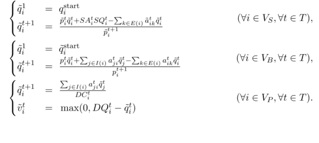
the optimal solution (˜ a, u, ˜ p) of the problem FFS( ˜ p, ¯ q), we can calculate the quality ˜ ¯ q and the

compensations v as follows,

 



˜

q _i ¹ = q ^start _i

˜

q _i ^t+1 = ^{p ˜}

t

i

q ˜

+SA

SQ

k∈E(i)

˜ a

q ˜

˜ p

( ∀ i ∈ V S , ∀ t ∈ T ),

 



˜

q _i ¹ = ˜ q ^start _i

˜

q _i ^t+1 = ^p

t i

q ˜

+

j∈I(i)

a

q ˜

k∈E(i)

a

q ˜

p

( ∀ i ∈ V _B , ∀ t ∈ T ),

 



˜ q _i ^t+1 =

∑

j∈I(i)

a

q ˜

DC

˜

v ^t _i = max(0, DQ ^t _i − q ˜ _i ^t )

( ∀ i ∈ V P , ∀ t ∈ T ).

3.6 Summary of the proposed approach

We summarize the relations among the problems defined in Subsections 3.1 to 3.4 in Fig.2.

Figure 2: Relations among the problems

Moreover, the following inequalities hold for the optimum values of the problems.

min(P) = min(P-POP) ≥ min(P-POP) = min(P-POP _v ) ≥ min(SDR (P-POP _v )) ≥ min(SDR (P-POP)), where min(P) denotes the optimum value of the problem (P). Note that the inequality min(SDR (P-POP)) ≥ min(SDR (P-POP)) does not always hold.

Now, we give the concrete algorithm as follows.

Proposed Algorithm

Step 0: Set J

= ∅ , J

= { (i, j, t) | (i, j) ∈ A, t ∈ T } , and choose a small ϵ > 0 such that ϵ < min

L

.

Step 1: Solve the SDP relaxation problem for NPP(J

, J

) with some valid inequalities men- tioned in Subsection 3.4, and obtain its solution (¯ a, p, ¯ q, ¯ v). ¯

Step 2: Let ¯ J

= { (i, j, t) ∈ J

| a

≤ ϵ } . If ¯ J

is not empty, then set J

= J

∪ J ¯

and J

= J

\ J ¯

, and go to Step 1.

Step 3: Solve FFS( p, ¯ q) defined in Subsection 3.5, and obtain a feasible solution (˜ ¯ a, p, ˜ q, ˜ v) of ˜ the original problem.

Step 4: Obtain a local optimal solution (a

, p

, q

, v

) by a general nonlinear programming solver starting from the feasible solution (˜ a, p, ˜ q, ˜ v)． ˜

The feasible solution (˜ a, p, ˜ q, ˜ v) obtained in Step 3 is not necessarily a local optimum for the ˜ pooling problem with the binary variables fixed. Thus, in Step 4, we solve the problem by some local search method.

4 Numerical Experiments

In this section, we present some numerical experiments with the proposed method. The experi- ments were carried out for eight problems. The network systems of the problems are presented in Figs. 3-6 and the given constants are shown in Tables 9-16. The numbers of their components, discretized time horizons and pipelines are shown in Table 2.

Figure 3: Problems 1, 2 Figure 4: Problems 3, 4

Problems 1 and 2 have the same network system, while they have different time horizons and

constants. Similarly, Problems 3 and 4 have different time horizons and the same network. Note

that their network is different from that of Problems 1 and 2. Problems 1-4 have only two

BlendTanks. Since the requirement of Plant is always positive, one of the tanks should send

the final products to the Plant. Thus the pipelines between the tanks are not used due to the

constraints (10). On the other hand, Problems 5-8 have more than three BlendTanks. Thus,

they may have flows between each pair of BlendTanks. Problems 7 and 8 are relatively large