RIMS-1783
Quenched Invariance Principles
for Random Walks and Elliptic Diffusions in Random Media with Boundary
By
Zhen-Qing CHEN, David A. CROYDON and Takashi KUMAGAI
May 2013
R ESEARCH I NSTITUTE FOR M ATHEMATICAL S CIENCES
Quenched Invariance Principles
for Random Walks and Elliptic Di↵usions in Random Media with Boundary
Zhen-Qing Chen⇤, David A. Croydon and Takashi Kumagai† May 31, 2013
Abstract
Via a Dirichlet form extension theorem and making full use of two-sided heat kernel estimates, we establish quenched invariance principles for random walks in random environments with a boundary. In particular, we prove that the random walk on a supercritical percolation cluster or amongst random conductances bounded uniformly from below in a half-space, quarter-space, etc., converges when rescaled di↵usively to a reflecting Brownian motion, which has been one of the important open problems in this area. We establish a similar result for the random conductance model in a box, which allows us to improve existing asymptotic estimates for the relevant mixing time. Furthermore, in the uniformly elliptic case, we present quenched invariance principles for domains with more general boundaries.
AMS 2000 Mathematics Subject Classification: Primary 60K37, 60F17; Secondary 31C25, 35K08, 82C41.
Keywords: quenched invariance principle, Dirichlet form, heat kernel, supercritical percolation, random conductance model
Running title: Quenched invariance principles for random media with a boundary.
1 Introduction
Invariance principles for random walks ind-dimensional reversible random environments date back to the 1980s [27, 40, 42, 43]. The most robust of the early results in this area concerned scaling limits for the annealed law, that is, the distribution of the random walk averaged over the possible realizations of the environment, or possibly established a slightly stronger statement involving some form of convergence in probability. Studying the behavior of the random walks under the quenched law, that is, for a fixed realization of the environment, has proved to be a much more difficult task, especially when there is some degeneracy in the model. This is because it is often the case that a typical environment has ‘bad’ regions that need to be controlled. Nevertheless, over the last
⇤Research partially supported by NSF Grants NSF Grant DMS-1206276, and NNSFC Grant 11128101.
†Research partially supported by the Grant-in-Aid for Scientific Research (B) 22340017 and (A) 25247007.
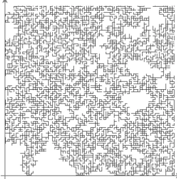
Figure 1: A section of the unique infinite cluster for supercritical percolation onZ2+with parameter p= 0.52.
decade significant work has been accomplished in this direction. Indeed, in the important case of the random walk on the unique infinite cluster of supercritical (bond) percolation onZd, building on the detailed transition density estimates of [6], a Brownian motion scaling limit has now been established [15, 46, 52]. Additionally, a number of extensions to more general random conductance models have also been proved [3, 8, 17, 45].
Whilst the above body of work provides some powerful techniques for overcoming the technical challenges involved in proving quenched invariance principles, such as studying ‘the environment viewed from the particle’ or the ‘harmonic corrector’ for the walk (see [16] for a survey of the recent developments in the area), these are not without their limitations. Most notably, at some point, the arguments applied all depend in a fundamental way on the translation invariance or ergodicity under random walk transitions of the environment. As a consequence, some natural variations of the problem are not covered. Consider, for example, supercritical percolation in a half-space Z+⇥Zd 1, or possibly an orthant of Zd. Again, there is a unique infinite cluster (Figure 1 shows a simulation of such in the first quadrant ofZ2), upon which one can define a random walk. Given the invariance principle for percolation onZd, one would reasonably expect that this process would converge, when rescaled di↵usively, to a Brownian motion reflected at the boundary. After all, as is illustrated in the figure, the ‘holes’ in the percolation cluster that are in contact with the boundary are only on the same scale as those away from it. However, the presence of a boundary means that the translation invariance/ergodicity properties necessary for applying the existing arguments are lacking. For this reason, it has been one of the important open problems in this area to prove the quenched invariance principle for random walk on a percolation cluster, or amongst random
conductances more generally, in a half-space (see [15, Section B] and [16, Problem 1.9]). Our aim is to provide a new approach for overcoming this issue, and thereby establish invariance principles within some general framework that includes examples such as those just described.
The approach of this paper is inspired by that of [19, 20], where the invariance principle for random walk on grids inside a given Euclidean domainD is studied. It is shown first in [19] for a class of bounded domains including Lipschitz domains and then in [20] foranybounded domainD that the simple random walk converges to the (normally) reflecting Brownian motion on D when the mesh size of the grid tends to zero. Heuristically, the normally reflecting Brownian motion is a continuous Markov process on D that behaves like Brownian motion in D and is ‘pushed back’
instantaneously along the inward normal direction when it hits the boundary. See Section 2 for a precise definition and more details. The main idea and approach of [19, 20] is as follows: (i) show that random walk killed upon hitting the boundary converges weakly to the absorbing Brownian motion in D, which is trivial; (ii) establish tightness for the law of random walks; (iii) show any sequential limit is a symmetric Markov process and can be identified with reflecting Brownian motion via a Dirichlet form characterization. In [19, 20], (ii) is achieved by using a forward- backward martingale decomposition of the process and the identification in (iii) is accomplished by using a result from the boundary theory of Dirichlet form, which says that the reflecting Brownian motion on D is the maximal Silverstein’s extension of the absorbing Brownian motion in D; see [19, Theorem 1.1] and [23, Theorem 6.6.9].
For quenched invariance principles for random walks in random environments with a boundary, step (i) above can be established by applying a quenched invariance principle for the full-space case.
For step (ii), i.e. establishing tightness, the forward-backward martingale decomposition method does not work well with unbounded random conductances. To overcome this difficulty, as well as for the desire to establish an invariance principle for every starting point, we will make the full use of detailed two-sided heat kernel estimates for random walk on random clusters. In particular, we provide sufficient conditions for the subsequential convergence that involve the H¨older continuity of harmonic functions (see Section 2.2). This continuity property can be verified in examples by using existing two-sided heat kernel bounds. We remark that the corrector-type methods for full- space models, such as the approach of [15], often require only upper bounds on the heat kernel.
Using the H¨older regularity, we can further show that any subsequential limit of random walks in random environments is a conservative symmetric Hunt process with continuous sample paths. In step (iii), we can identify the subsequential limit process with the reflecting Brownian motion by a Dirichlet form argument (see Theorem 2.1). In summary, our approach for proving quenched invariance principles for random walks in random environments with a boundary encompasses two novel aspects: a Dirichlet form extension argument and the full use of detailed heat kernel estimates.
The full generality of the random conductance model to which we are able to apply the above argument is presented in Section 3. As an illustrative application of Theorem 2.1, though, we state here a theorem that verifies the conjecture described above concerning the di↵usive behavior of the random walk on a supercritical percolation cluster on a half-space, quarter-space, etc. We recall that the variable speed random walk (VSRW) on a connected (unweighted) graph is the continuous time Markov process that jumps from a vertex at a rate equal to its degree to a uniformly chosen neighbor (see Section 3 for further details). In this setting, similar results to that stated can be
obtained for the so-called constant speed random walk (CSRW), which has mean one exponential holding times, or the discrete time random walk (see Remark 3.18 below).
Theorem 1.1. Fix d1, d2 2Z+ such thatd1 1 andd:=d1+d2 2. LetC1 be the unique infinite cluster of a supercritical bond percolation process onZd+1⇥Zd2, and letY = (Yt)t 0 be the associated VSRW. For almost-every realization of C1, it holds that the rescaled process Yn = (Ytn)t 0, as defined by
Ytn:=n 1Yn2t,
started fromY0n=xn2n 1C1, wherexn!x2Rd+1⇥Rd2, converges in distribution to{Xct;t 0}, where c2(0,1) is a deterministic constant and{Xt;t 0} is the (normally) reflecting Brownian motion on Rd+1 ⇥Rd2 started fromx.
As an alternative to unbounded domains, one could consider compact limiting sets, replacingYn in the previous theorem by the rescaled version of the variable speed random walk on the largest percolation cluster contained in a box [ n, n]d\Zd, for example. As presented in Section 4.1, another application of Theorem 2.1 allows an invariance principle to be established in this case as well, with the limiting process being Brownian motion in the box [ 1,1]d, reflected at the boundary.
Consequently, we are able to refine the existing knowledge of the mixing time asymptotics for the sequence of random graphs in question from a tightness result [13] to an almost-sure convergence one (see Corollary 4.4 below).
Note that the analytical part of our results (namely Section 2) holds for a large class of possibly non-smooth domains, called uniform domains, which include (global) Lipschitz domains and the classical van Koch snowflake planar domain as special cases. Although in the percolation setting we only consider relatively simple domains with ‘flat’ boundaries, this is mainly for technical reasons so that deriving the percolation estimates in Section 3.1 required for our proofs is manageable.
Indeed, in the case when we restrict to uniformly elliptic random conductances, so that controlling the clusters of extreme conductances is no longer an issue, we are able to derive from Theorem 2.1 quenched invariance principles in any uniform domain. These are discussed in Section 4.2.
Moreover, in Section 4.3 we explain how the same techniques can be applied in the uniformly elliptic random divergence form setting. (We refer to [41, 38] and the references therein for the history of homogenization for di↵usions in random environments.)
The remainder of the paper is organized as follows. In Section 2, we introduce an abstract framework for proving invariance principles for reversible Markov processes in a Euclidean domain.
This is applied in Section 3 to our main example of a random conductance model in half-spaces, quarter-spaces, etc. The details of the other examples discussed above are presented in Section 4. Our results for the random conductance model depend on a number of technical percolation estimates, some of the proofs of which are contained in the appendix that appears at the end of this article. Finally, the appendix also contains a proof of a generalization of existing quenched invariance principles that allows for arbitrary starting points (previous results have always started the relevant processes from the origin, which will not be enough for our purposes).
Finally, in this paper, for a locally compact separable metric spaceE, we useCb(E) andC1(E) to denote the space of bounded continuous functions on E and the space of continuous functions on E that vanish at infinity, respectively. The space of continuous functions on E with compact
support will be denoted byCc(E). For real numbers a, b, we usea_b anda^bfor max{a, b} and min{a, b}, respectively.
2 Framework
The following definition is taken from V¨ais¨al¨a [55], where various equivalent definitions are dis- cussed. An open connected subset DofRd is calleduniformif there exists a constantC such that for every x, y 2 D there is a rectifiable curve joining x and y in D with length( ) C|x y| and moreover min{|x z|,|z y|} Cdist(z, @D) for all points z 2 . Here dist(z, @D) is the Euclidean distance between the pointzand the set@D. Note that a uniform domain is calledinner uniformin [35, Definition 3.6].
For example, the classical van Koch snowflake domain in the conformal mapping theory is a uniform domain in R2. Every (global) Lipschitz domain is uniform, and every non-tangentially accessible domaindefined by Jerison and Kenig in [37] is a uniform domain (see (3.4) of [37]). How- ever, the boundary of a uniform domain can be highly nonrectifiable and, in general, no regularity of its boundary can be inferred (besides the easy fact that the Hausdor↵dimension of the boundary is strictly less than d).
It is known (see Example 4 on page 30 and Proposition 1 in Chapter VIII of [39]) that any uniform domain in Rdhasm(@D) = 0 and there exists a positive constant c >0 such that
m(D\B(x, r)) c rn for all x2D and 0< r1, (2.1) wherem denotes the Lebesgue measure inRd.
LetDbe a uniform domain inRd. Suppose (A(x))x2D is a measurable symmetricd⇥dmatrix- valued function such that
c 1I A(x)cI for a.e. x2D, (2.2)
whereI is the d-dimensional identity matrix andc is a constant in [1,1). Let E(f, g) := 1
2 Z
Drf(x)·A(x)rg(x)dx forf, g2W1,2(D), (2.3) where
W1,2(D) := f 2L2(D;m) : rf 2L2(D;m) .
An important property of a uniform domain D ⇢ Rd is that there is a bounded linear extension operator T :W1,2(D) ! W1,2(Rd) such that T f =f a.e. on D for f 2W1,2(D). It follows that (E, W1,2(D)) is a regular Dirichlet form onL2(D;m) and so there is a continuous di↵usion process X= (Xt, t 0;Px, x2D) associated with it, starting fromE-quasi-every point. Here a property is said to holdE-quasi-everywhere means that there is a setN ⇢Dhaving zero capacity with respect to the Dirichlet form (E, W1,2(D)) so that the property holds for points in Nc. According to [35, Theorem 3.10] and (2.1) (see also [12, (3.6)]) X admits a jointly continuous transition density functionp(t, x, y) on R+⇥D⇥D and
c1t d/2exp
✓ c2|x y|2 t
◆
p(t, x, y)c3t d/2exp
✓ c4|x y|2 t
◆
(2.4)
for every x, y 2 D and 0 < t 1. Here the constants c1,· · · , c4 > 0 depend on the di↵usion matrixA(x) only through the ellipticity bound cin (2.2). Consequently, X can be refined so that it can start from every point in D. The process X is called a symmetric reflecting di↵usion on D. We refer to [21] for sample path properties of X. When A=I,X is the (normally) reflecting Brownian motion on D. Reflecting Brownian motion X on D in general does not need to be semimartingale. When@Dlocally has finite lower Minkowski content, which is the case when Dis a Lipschitz domain, X is a semimartingale and admits the following Skorohod decomposition (see [22, Theorem 2.6]):
Xt=X0+Wt+ Z t
0
~n(Xs)dLs, t 0. (2.5)
Here W is the standard Brownian motion in Rd, ~n is the unit inward normal vector field of D on @D, and L is a positive continuous additive functional of X that increases only when X is on the boundary, that is, Lt = Rt
01{Xs2@D}dLs for t 0. Moreover, it is known that the reflecting Brownian motion spends zero Lebesgue amount of time at the boundary@D. These together with (2.5) justify the heuristic description we gave in the introduction for the reflecting Brownian motion inD.
2.1 Convergence to reflecting di↵usion
In this subsection,Dis a uniform domain inRd andXis a reflecting di↵usion process onDassoci- ated with the Dirichlet form (E, W1,2(D)) onL2(D;m) given by (2.3). Denote by (XD,PDx, x2D) the subprocess ofX killed on exitingD. It is known (see, e.g., [23]) that the Dirichlet form of XD on L2(D;m) is (E, W01,2(D)), where
W01,2(D) := f 2W1,2(D) : f = 0 E-quasi-everywhere on @D .
Suppose that {Dn;n 1} is a sequence of Borel subsets of D such that each Dn supports a measure mn that converges vaguely to the Lebesgue measure m on D. The following result plays a key role in our approach to the quenched invariance principle for random walks in random environments with boundary.
Theorem 2.1. For each n 2 N, let (Xn,Pnx, x 2 Dn) be an mn-symmetric Hunt process on Dn. Assume that for every subsequence {nj}, there exists a sub-subsequence {nj(k)} and a continu- ous conservative m-symmetric strong Markov process (X,e ePx, x2 D) such that the following three conditions are satisfied:
(i) for every xnj(k) !x withxnj(k) 2Dnj(k), Pnxnj(k)j(k) converges weakly in D([0,1), D) to ePx; (ii) XeD, the subprocess of Xe killed upon leavingD, has the same distribution as XD; (iii) the Dirichlet form ( ˜E,F˜) of Xe onL2(D;m) has the properties that
C⇢F˜ and E˜(f, f)C0E(f, f) for every f 2C, (2.6) where C is a core for the Dirichlet form (E, W1,2(D))and C02[1,1) is a constant.
It then holds that for every xn ! x with xn 2Dn, (Xn,Pnxn) converges weakly in D([0,1), D) to (X,Px).
Proof. With both Xe and X being m-symmetric Hunt processes on D, it suffices to show that their corresponding (quasi-regular) Dirichlet forms on L2(D;m) are the same; that is (Ee,Fe) = (E, W1,2(D)). Condition (iii) immediately implies that W1,2(D)⇢Fe and
Ee(f, f)C0E(f, f) for every f 2W1,2(D).
Next, observe that sinceXe is a di↵usion process admitting no killings, its associated Dirichlet form is strongly local. Thus for every u 2 Fe, Ee(u, u) = 12µehui(D), where µehui is the energy measure corresponding tou. By the proof of [47, Proposition on page 389] ,
e
µhui(dx)C0ru(x)A(x)ru(x)dxcC0|ru(x)|2dx on D for every u2W1,2(D).
This in particular implies that e
µhui(@D) = 0 foru2W1,2(D). (2.7)
On the other hand, by the strong local property of µehui and the fact that XeD has the same distribution asXD, we have that every bounded function in Fe– the collection of which we denote by Feb – is locally inW01,2(D) and
1D(x)µehui(dx) =1D(x)ru(x)A(x)ru(x)dx foru2Feb. (2.8) This together with (2.7) implies thatEe(u, u) =E(u, u) for every bounded u2W1,2(D), and hence for every u 2 W1,2(D). Furthermore, (2.8) implies that for u 2 Feb, R
D|ru(x)|2dx < 1 and so u2W1,2(D). Consequently we have Fe⇢W1,2(D) and thus (Ee,Fe) = (E, W1,2(D)).
Remark 2.2. (i) Note that if (Xtn)t 0 is conservative for eachn2N and {Pnxj(k)nj(k)} is tight, then X˜ is conservative.
(ii) Theorem 2.1 can be viewed as a variation of [19, Theorem 1.1]. The di↵erence is that in [19, Theorem 1.1], the constantC0 in (2.6) is assumed to be 1 but the limiting processXe only need to be Markov and does not need to be continuous a priori, while for Theorem 2.1, the condition on the constantC0 is weaker but we need to assume a priori that the limit process Xe is continuous.
2.2 Sufficient condition for subsequential convergence
In this subsection, we give some sufficient conditions for the subsequential convergence of{Xn}; in other words, sufficient conditions for (i) in Theorem 2.1. For simplicity, we assume that 02Dnfor all n 1 throughout this section, though note this restriction can easily be removed.
We start by introducing our first main assumption, which will allow us to check an equi- continuity property for the -potentials associated with the elements of{Xn}(see Proposition 2.4 below). In the statement of the assumption, we suppose that ( n)n 1 is a decreasing sequence in [0,1] with limn!1 n= 0 and such that|x y| n for all distinct x, y2Dn. (When n⌘0, this condition always holds. However, our assumption will give an additional restriction.) We denote by B(x, r) the Euclidean ball of radius r centered at x, and ⌧A(Xn) the first exit time of the process Xn from the setA.
Assumption 2.3. There existc1, c2, c3, , 2(0,1), N0 2N such that the following hold for all n N0, x0 2B(0, c1n1/2), and n1/2r1.
(i) For all x2B(x0, r/2)\Dn,
Enx
⇥⌧B(x0,r)\Dn(Xn)⇤
c2r .
(ii) If hn is bounded in Dn and harmonic (with respect to Xn) in a ball B(x0, r), then
|hn(x) hn(y)|c3
✓|x y| r
◆
khnk1 for x, y2B(x0, r/2)\Dn.
Define for >0 the -potential Unf(x) =Enx
Z 1
0
e tf(Xtn)dt forx2Dn.
Proposition 2.4. Under Assumption 2.3 there exist C =C 2(0,1) and 0 2 (0,1) such that the following holds for any bounded functionf onDn, for anyn N0 and anyx, y2Dn such that x2B(0, c1n1/2) and |x y|<1/4:
|Unf(x) Unf(y)|C|x y| 0kfk1. (2.9) In particular, we have
lim!0 sup
n N0
sup
x,y2Dn\B(0,c1n1/2):
|x y|<
|Unf(x) Unf(y)|= 0. (2.10)
Proof. The proof is similar to that of [11, Proposition 3.3]. Fix x0 2B(0, c1n1/2)\Dn, let 1 r
n1/2, and supposex, y2B(x0, r/2). Set⌧rn:=⌧B(x0,r)\Dn(Xn). By the strong Markov property, Unf(x) = Enx
Z ⌧rn 0
e tf(Xtn)dt+Enx
h(e ⌧rn 1)Unf(X⌧nn r)i
+Enx
hUnf(X⌧nn r)i
= I1+I2+I3,
and similarly when xis replaced by y. We have by Assumption 2.3(i) that
|I1| kfk1Enx⌧rnc2r kfk1, and by notingkUnfk1 1kfk1 that
|I2| Enx⌧rnkUnfk1c2r kfk1. Similar statements also hold when x is replaced byy. So,
Unf(x) Unf(y) 4c2r kfk1+ EnxUnf(X⌧nn
r) EnyUnf(X⌧nn
r) . (2.11)
But z ! EnzUnf(X⌧nn
r) is bounded in Rd and harmonic in B(x0, r), so by Assumption 2.3(ii), the second term in (2.11) is bounded by c3(|x y|/r) kUnfk1. So by kUnfk1 1kfk1 again, we have
Unf(x) Unf(y) c
✓
r + 1
✓|x y| r
◆ ◆
kfk1 forx, y2B(x0, r/2). (2.12) Now, for distinct x, y 2Dn with x2B(0, c1n1/2) and ( n1/2)2 |x y|<1/4 (note that since
|x y| n for distinct x and y, the first inequality always hold), let x0 = x and r =|x y|1/2. Then nr <1/2 andy2B(x0, r/2) (because |x0 y|=r2 < r/2). Thus we can apply (2.12) to obtain
Unf(x) Unf(y) c⇣
|x y| /2+ 1|x y| /2⌘ kfk1
c(1 + 1)|x y|( ^ )/2kfk1.
So (2.9) holds with C = c(1 + 1) and 0 = ( ^ )/2. The result at (2.10) is immediate from (2.9).
We note that with an additional mild condition, we can further obtain equi-H¨older continuity of the associated semigroup. (The next proposition will only be used in the proof of Theorem 3.13 below.) Set BR := B(0, R)\Dn for R 2 [2,1). Denote by Xn,BR the subprocess of Xn killed upon exiting BR, and {Ptn,BR;t 0} the transition semigroup of Xn,BR. (When R = 1, we set (Ptn)t 0 := (Ptn,B1)t 0, i.e. the semigroup ofXn itself.) Forp2[1,1], we usek·kp,n,R to denote theLp-norm with respect to mn on BR.
Proposition 2.5. Let R 2 [2,1] and t > 0. Suppose there exist c1 > 0 and N1 2 N (that may depend on R and t) such that for every g2L1(BR, mn),
kPtn,BRgk1,n,Rc1kgk1,n,R, for all n N1.
Suppose in addition that Assumption 2.3 holds with Xn,BR andBR in place ofXn and Dn, respec- tively. It then holds that there exist constants c2(0,1) and N2 1 (that also may depend on R and t) such that
Ptn,BRf(x) Ptn,BRf(y) c2|x y| 0kfk2,n,R,
for every n N2, f 2 L2(BR;mn), and mn-a.e. x, y 2 BR/2 with |x y| < 1/4. Here 0 is the constant of Proposition 2.4.
Proof. We follow [11, Proposition 3.4]. For notational simplicity, we drop the sufficesn N0 and BR throughout the proof. Using spectral representation theorem for self-adjoint operators, there exist projection operators Eµ=Eµn,R on the space L2(BR;mn) such that
f = Z 1
0
dEµ(f), Ptf = Z 1
0
e µtdEµ(f), U f = Z 1
0
1
+µdEµ(f). (2.13) Define
h= Z 1
0
( +µ)e µtdEµ(f).
Since supµ( +µ)2e 2µtc, we have khk22 =
Z 1
0
( +µ)2e 2µtdhEµ(f), Eµ(f)i c Z 1
0
dhEµ(f), Eµ(f)i=ckfk22,
where for f, g2L2,hf, gi is the inner product off and g inL2. Thush is a well defined function inL2.
Now, supposeg2L1. By the assumption,kPtgk1ckgk1, from which it follows thatkPtgk2 ckgk1. Since supµ( +µ)e µt/2c, using Cauchy-Schwarz we have
hh, gi= Z 1
0
( +µ)e µtdhEµ(f), gi
✓Z 1
0
( +µ)e µtdhEµ(f), f)i
◆1/2✓Z 1
0
( +µ)e µtdhEµ(g), gi
◆1/2
c
✓Z 1
0
dhEµ(f), fi
◆1/2✓Z 1
0
e µt/2dhEµ(g), gi
◆1/2
=ckfk2kPt/2gk2 c0kfk2kgk1.
Taking the supremum overg2L1 withL1 norm less than 1, this yieldskhk1ckfk2. Finally, by (2.13),
U h= Z 1
0
e µtdEµ(f) =Ptf, a.e., and so the H¨older continuity ofPtf follows from Proposition 2.4.)
Let D(R+, D) be the space of right continuous functions on R+ having left limits and taking values in D that is equipped with the Skorohod topology. For t 0, we use Xt to denote the coordinate projection map onD(R+, D); that is,Xt(!) =!(t) for!2D(R+, D). For subsequential convergence to a di↵usion, we need the following.
Assumption 2.6. (i) For any sequence xn!x with xn2Dn,{Pnxn} is tight in D(R+, D).
(ii) For any sequencexn!x withxn2Dn and any ">0, lim!0lim sup
n!1 Pnxn(J(Xn, )>") = 0, where J(X, ) :=R1
0 e u 1^sup tu|Xt Xt | du.
We need the following well-known fact (see, for example [7, Lemma 6.4]) in the proof of Propo- sition 2.8. For readers’ convenience, we provide a proof here.
Lemma 2.7. Let K be a compact subset of Rd. Supposef andfk,k2N, are functions onK such that limk!1fk(yk) = f(y) whenever yk 2 K converges to y. Then f is continuous on K and fk converges to f uniformly on K.
Proof. We first show that f is continuous on K. Fix x0 2K. Let xk be any sequence in K that converges to it. Since limi!1fi(x) = f(x) for every x 2 K, there is a sequence nk 2 N that
increases to infinity so that|fnk(xk) f(xk)|2 kfor everyk 1. Since limk!1fnk(xk) =f(x0), it follows that limk!1|f(x0) f(xk)|= 0. This shows thatf is continuous atx0 and hence onK.
We next show thatfk converges uniformly tof onK. Suppose not. Then there is">0 so that for everyk 1, there arenk kandxnk 2K so that|fnk(xnk) f(xnk)|>". SinceK is compact, by selecting a subsequence if necessary, we may assume without loss of generality thatxnk !x0 2 K. As limk!1fnk(xnk) =f(x0) by the assumption, we have lim infk!1|f(x0) f(xnk)| ". This contradicts to the fact thatf is continuous onK.
Now, applying the argument in [7, Section 6], we can prove that any subsequential limit of the laws of Xn under Pnxn is the law of a symmetric di↵usion. For this, we need to introduce a projection map from D to Dn. For each n 1, let n : D ! Dn be a map that projects each x 2 D to some n(x) 2 Dn that minimizes |x y| over y 2 Dn (if there is more than one such point that does this, we choose and fix one). If needed, we extend a function f defined on Dn to be a function onD by settingf(x) =f( n(x)). Note that eachDn supports the measure mn that converges vaguely to m. This implies that for each x 2 D and r > 0, there is an N 1 so that
n(x)2B(x, r) for everyn N. From this, one concludes that
n(xn)!x0 for every sequencexn2D that converges tox0. (2.14) Proposition 2.8. Suppose that Assumptions 2.3 and 2.6 hold and that {Xn,Pnx, x 2 Dn} is conservative for sufficiently large n. For every subsequence {nj}, there exists a sub-subsequence {nj(k)} and a continuous conservative m-symmetric Hunt process (X,e Pex, x 2 D) such that for every xnj(k) !x, Pnxj(k)nj(k) converges weakly in D([0,1), D) to ePx.
Proof. For notational simplicity, let us relabel the subsequence as {n}. We first claim that there exists a (sub-)subsequence{nj}such thatUnjf converges uniformly on compact sets for each >0 and f 2Cb(D). Indeed, let { i} be a dense subset of (0,1) and {fk} a sequence of functions in Cb(D) such that kfkk1 1 and whose linear span is dense in (Cb(D),k·k1). For fixed m and i, by Proposition 2.4 and the Ascoli-Arzel`a theorem, there is a subsequence ofUnifk that converges uniformly on compact sets. By a diagonal selection procedure, we can choose a subsequence{nj} such that Unjifk converges uniformly on compact sets for every m and i to a H¨older continuous function which we denote as U ifk. Noting that
Un Un = ( )UnUn, kUnk1!1 1
, kUn Unk1!1 , (2.15) a careful limiting argument shows thatUnjf converges uniformly on compact sets, say to U f, for any >0 and any continuous functionf, and (2.15) holds as well for{U }. By the equi-continuity of Unjf , we also have Unjf(xnj)!U f(x) for eachxnj 2Dnj that converges to x2D.
We next claim that Pnxnjj converges weakly, say to Pex. Indeed, by Assumption 2.6(i), {Pnxjnj} is tight, so it suffices to show that any two limit points agree. Let P0 and P00 be any two limit points.
Then, one sees that
E0Z 1
0
e sf(Xs)ds =U f(x) =E00Z 1
0
e sf(Xs)ds ,
for anyf 2Cb(D). So, by the uniqueness of the Laplace transform, E0[f(Xs)] =E00[f(Xs)]
for almost all s 0 and hence for every s 0 since s ! Xs is right continuous. So the one- dimensional distributions of Xt under P0 and P00 are the same. Set Psf(x) := E0f(Xs). We have Psnjf(xnj) ! Psf(x) for every sequence xnj 2 Dnj that converges to x. Recall the restriction map n introduced proceeding the statement of this theorem. It follows from (2.14) that Psnj(f
nj)(ynj)!Psf(y) for every sequenceynj 2Dthat converges to y. Thus by Lemma 2.7, Psnj(f
nj) converges to Psf uniformly on compact subsets of Dand Psf 2Cb(D) for every f 2Cc(D).
Forf, g2Cc(D) and 0s < t, by the Markov property ofX underPnxnjj , Enxjnj[g(Xs)f(Xt)] = Enxjnj ⇥
((Pt sn f)g)(Xs)⇤
= Enxjnj [((Pt sf)g)(Xs)] +Enxnjj ⇥
((Pt sn f Pt sf)g)(Xs)⇤ .
The first term of the right-hand side converges to E0[((Pt sf)g)(Xs)] by the above proof, while the second term goes to 0 since Pt snj f ! Pt sf uniformly on compact sets. Repeating this, we conclude that for everyk 1 and every 0< s1 < s2<· · ·< sk and fj 2Cc(D),
E0 2 4
Yk j=1
fj(Xsj) 3 5=E00
2 4
Yk j=1
fj(Xsj) 3
5=Ps1(f1Ps2 s1(f2Ps3 s2(f3· · ·))) (x). (2.16)
This proves that the finite dimensional distributions of X under P0 and P00 are the same. Conse- quently, P0 = P00, which we now denote as Pex. Moreover, (2.16) shows that (X,Pex, x 2 D) is a Markov process with transition semigroup {Pt, t 0}.
Next we show that {ePx:x2D}is a strong Markov process. Note that X is conservative with ePx(X0 = x) = 1, and under Assumption 2.6(ii), Xt is continuous a.s. under ePx. We also have Ptf 2 Cb(D) for f 2Cc(D). It is easy to deduce from these properties and (2.16) that for every f 2Cc(D) and every stopping time T,
Ex[f(XT+t)|FT+] =Ptf(XT), x2D.
See the proof of Theorem 2.3.1 on p.56 of [24]. From it, one gets the strong Markov property ofX by a standard measure-theoretic argument (see p.57 of [24]). SinceX is continuous and has infinite lifetime, this in fact shows that X is a continuous conservative Hunt process.
Finally, forf, g2Cc(D), by the convergence of semigroups and vague convergence of measures, it holds that, for everyt >0,
Z
Dn
(Ptnjf)(x)g(x)mnj(dx)! Z
D
(Ptf)(x)g(x)m(dx).
Since Xnj is mn-symmetric, this readily yields the desiredm-symmetry of ˜X.
Remark 2.9. Note that we did not use any special properties of the Euclidean metric in this section, so that all the arguments in this section can be extended to a metric measure space without any changes.
By Theorem 2.1, Remark 2.2 (i) and Proposition 2.8, we see that in order to prove (Xn,Pnxn) converges weakly to (X,Px) in D([0,1), D) as n ! 1, it suffices to verify condition (ii), (iii) in Theorem 2.1, vague convergence of the measure mn tom onD, Assumptions 2.3 and 2.6, and the conservativeness of (Xn,Pnxn) for eachn2N.
3 Random conductance model in unbounded domains
In this section we will obtain, as a first application of our theorem, a quenched invariance prin- ciple for random walk amongst random conductances on half-spaces, quarter-spaces, etc. The assumptions we make on the random conductances include the supercritical percolation model, and random conductances bounded uniformly from below and with finite first moments. For the main conclusion, see Theorem 3.17.
Fix d1, d2 2Z+. Let d:= d1+d2, and define a graph (L, EL) by setting L := Zd+1 ⇥Zd2 and EL :={e={x, y}: x, y 2L, |x y|= 1}. GivenO ✓EL, letC1(L,O) be the infinite connected cluster of (L,O), provided it exists and is unique (otherwise setC1(L,O) :=;).
Let µ= (µe)e2EL be a collection of independent and identically distributed random variables on [0,1), defined on a probability space (⌦,P) such that
p1 :=P(µe>0)> pbondc (Zd), (3.1) where pbondc (Zd) 2 (0,1) is the critical probability for bond percolation on Zd. We assume that there isc >0 so that
P(µe2(0, c)) = 0, (3.2)
and
E(µe)<1. (3.3)
This framework includes the special cases of supercritical percolation (where P(µe = 1) = p1 = 1 P(µe = 0)) and the random conductance model with conductances bounded from below (that is, P(cµe<1) = 1 for some c > 0) and having finite first moments. For each x 2 L, set µx=P
y⇠xµxy. Set
O1 :={e2EL :µe>0}, C1:=C1(L,O1).
Note that for the random conductance model bounded from below,C1=L.
For each realization of C1, there is a continuous time Markov chain Y = (Yt)t 0 on C1 with transition probabilitiesP(x, y) =µxy/µx, and the holding time at eachx2C1being the exponential distribution with mean µx1. Such a Markov chain is sometimes called a variable speed random walk (VSRW). The corresponding Dirichlet form is (E, L2(C1;⌫)), where ⌫ is the counting measure on C1 and
E(f, g) = 1 2
X
x,y2C1, x⇠y
(f(x) f(y))(g(x) g(y))µxy forf, g2L2(C1;⌫).
The corresponding discrete Laplace operator isLVf(x) =P
y(f(y) f(x))µxy. For each f, g that have finite support, we have
E(f, g) = X
x2C1
(LVf)(x)g(x).
We will establish a quenched invariance principle forY in Section 3.3, but we first need to derive some preliminary estimates regarding the geometry of C1 and the heat kernel associated with Y. 3.1 Percolation estimates
In this section, we derive a number of useful properties of the underlying percolation cluster C1. Most importantly, we introduce the concept of ‘good’ and ‘very good’ balls for the model and provide estimates for the probability of such occurring, see Definition 3.4 and Proposition 3.5 below.
Since a variety of percolation models will appear in the course of this paper, let us now make explicit that the critical probability for bond/site percolation on an infinite connected graph con- taining the vertex 0 is
pc := inf{p2[0,1] : Pp(0 is in an infinite connected cluster of open bonds/sites)>0}, where Pp is the law of parameter p bond/site percolation on the graph in question. Note in particular that the critical probability for bond percolation on Lis identical to pbondc (Zd), see [32, Theorem 7.2] (which is the bond percolation version of a result originally proved as [33, Theorem A]). Recall
O1 :={e2EL :µe>0}, C1:=C1(L,O1).
That C1 is non-empty almost-surely is guaranteed by [10, Corollary to Theorem 1.1] (this covers d 3, and, as is commented there, the cased= 2 can be tackled using techniques from [36]).
Now, suppose that µis actually a restriction of independent and identically distributed (under P) random variables (µe)e2EZd, where EZd are the usual nearest-neighbor edges for the integer latticeZd, and define
O˜1 :={e2EZd:µe>0}, C˜1 :=C1(Zd,O˜1).
For sufficiently largeK so that
q=q(K) :=P(0< µe< K 1) +P(µe> K)< p1 pbondc (Zd), and writing ˜OI :={e2EZd:µe 2I}forI ✓[0,1), we let
O˜R := O˜(0,K 1)[(K,1), O˜S := n
e2O˜1 :e\e0 6=; for somee02O˜R
o,
O˜2 := O˜1\O˜S.
We will also define O2:= ˜O2\EL, and setC2 :=C1(L,O2) – the next lemma will guarantee that this set is non-empty almost-surely.
To represent the set of ‘holes’, let H:=C1\C2. Moreover, forx2C1, letH(x) be the connected component of C1\C2 containing x. The following lemma provides control on the size of these components. Since its proof is a somewhat technical adaptation to our setting of that used to establish [3, Lemma 2.3], which dealt with the whole Zd model, we defer this to the appendix.
Note, though, that in the percolation case (i.e. when µe are Bernoulli random variables) or the uniformly elliptic random conductor case, the proof of the result is immediate; indeed, for large enoughK, we have that O2=O1, and so H=;.
Lemma 3.1. For sufficiently large K, the following holds.
(i) All the connected components of H are finite. Furthermore, there exist constants c1, c2 such that: for each x2L,
P(x2C1 and diam(H(x)) n)c1e c2n, where diam denotes the diameter with respect to the `1 metric on Zd.
(ii) There exists a constant ↵ such that, P-a.s., for large enough n, the volume of any hole inter- secting the box [ n, n]d\L is bounded above by(logn)↵.
In what follows, we will need to make comparisons between two graph metrics on (C1,O1), and the Euclidean metric. The first of these, d1, will simply be defined to be the shortest path metric on (C1,O1), considered as an unweighted graph. To define the second metric,d1, we follow [8] by defining edge weights
t(e) :=CA^µe1/2,
where CA < 1 is a deterministic constant, and then letting d1 be the shortest path metric on (C1,O1), considered as a weighted graph (in [8], the analogous metric was denoted ˜d). We note that the latter metric on C1 satisfies
CA2_µ{y,z} d1(x, y) d1(x, z) 2 1,
for anyx, y, z2C1with{y, z}2O1. Observe that, since the weightst(e) are bounded above byCA, we immediately have thatd1is bounded above byCAd1, Hence the following lemma establishes both d1 and d1 are comparable to the Euclidean one. An easy consequence of this is the comparability of balls in the di↵erent metrics, see Lemma 3.3. The proofs of both these results are deferred to the appendix.
Lemma 3.2. There exist constants c1, c2, c3 such that: forR 1, sup
x,y2L:
|x y|R
P(x, y2C1 and d1(x, y) c1R)c2e c3R, (3.4)
and also, for every x, y2L,
P x, y2C1 and d1(x, y)c11|x y| c2e c3|x y|. (3.5)
Lemma 3.3. There exist constants c1, c2, c3, c4 such that: for every x2L, R 1,
P {x2C1}\ C1\BE(x, c1R)✓B1(x, R)✓B1(x, CAR)✓BE(x, c2R) c c3e c4R, where B1(x, R) is a ball in the metric space (C1, d1), B1(x, R) is a ball in (C1, d1), and BE(x, R) is a Euclidean ball.
We continue by adapting a definition for ‘good’ and ‘very good’ balls from [3]. In preparation for this, we defineµ0e :=1{e2O1}, setµ0x :=P
y2Lµ0{x,y} forx2L, and then extendµ0 to a measure on L. Moreover, we set := 1 2(1 +d) 1.
Definition 3.4. (i) Let CV, CP, CW, CR, CD be fixed strictly positive constants. We say the pair (x, R)2C1⇥R+ isgood if:
B1(x, CA1r)✓B1(x, r)✓B1(x, CDr), 8r R, (3.6)
|y z| CR1R, 8y2B1(x, R/2), z2B1(x,8R/9)c, (3.7)
CVRdµ0(B1(x, R)), (3.8)
diam(H(y))R , 8y2BE(x, R)\C1, (3.9) and the weak Poincar´e inequality
X
y2B1(x,R)
f(y) fˇB1(x,R) 2µ0y CPR2 X
y,z2B1(x,CWR):
{y,z}2O1
|f(y) f(z)|2 (3.10)
holds for every f : B1(x, CWR) ! R. (Here fˇB1(x,R) is the value which minimizes the left-hand side of (3.10)).
(ii) We say a pair(x, R)2C1⇥R+ isvery goodif: there existsN =N(x,R) such that (y, r) is good whenever y2B1(x, R) andN rR. We can always assume that N 2. Moreover, if N M, we will say that (x, R) is M-very good.
(iii) Let ↵ 2 (0,1]. For x 2 C1, we define R(↵)x to be the smallest integer M such that (x, R) is R↵-very good for all R M. We set R(↵)x = 0 if x62C1.
The following proposition, which is an adaptation of [3, Proposition 2.8], provides bounds for the probabilities of these events and for the distribution ofRx(↵).
Proposition 3.5. There exist c1, c2, CV, CP, CW, CR, CD (depending on the law of µ and the di- mension d) such that the following holds. For x2L, R 1, ↵2(0,1],
P(x2C1, (x, R) is not good)c1e c2R , (3.11) P(x2C1, (x, R) is notR↵-very good)c1e c2R↵ . (3.12) Hence
P⇣
x2C1, R(↵)x n⌘
c1e c2n↵ . (3.13)
Proof. That
P(x2C1, (3.6) does not hold)c3e c4R is a straightforward consequence of Lemma 3.3.
For the second property, we have P(x2C1, (3.7) does not hold)
= P x2C1, 9y2B1(x, R/2), z2B1(x,8R/9)c : |y z|< CR1R
P x2C1, 9y2BE(x, c5R)\B1(x, R/2), z2B1(x,8R/9)c: |y z|< CR1R +c6e c7R
c6e c7R+ X
y2BE(x,c5R)
X
z2BE(y,CR1R)
P y, z2C1, d1(y, z)> R/3
c8e c9R
where we apply Lemma 3.3 to deduce the first inequality, and (3.4) to obtain the final one.
For (3.8), applying Lemma 3.3 again yields P(x2C1, (3.8) does not hold)
= P⇣
x2C1, µ0(B1(x, R))< CVRd⌘
c10e c11R+P⇣
x2C1, |C1\BE(x, c12R)|< CVRd⌘ .
Now, letQ ✓BE(x, c12R)\L be a cube of side-length c13R such that infy2L\Q|x y| c13R/2.
Moreover, if we letC+(Q) be the largest connected component of the graph (Q,O1), then P(x2C1, (3.8) does not hold)
P⇣
x2C1\C+(Q), |C1\Q|< CVRd⌘
+P x2C1\C+(Q) +c10e c11R
P⇣
|C+(Q)|< CVRd⌘ +P⇣
x2C˜1\C+(Q)⌘
+c10e c11R.
This bound is now expressed in terms of the fullZdmodel, for which appropriate estimates already exist. In particular, the first term here is bounded above by P(G(Q)c), where G(Q) is the event that |C+(Q)| 12P(02C˜1)|Q|(recall that ˜C1 :=C1(Zd,O˜1)). Consequently, by simply translating the relevant part of [3, Lemma 2.6] to our setting (taking K =1), we obtain that it is bounded above by c13e c14R . That the second term is bounded above by c15e c16R can be established by applying [6, Lemma 2.8].
To check the fourth property, we simply note P(x2C1, (3.9) does not hold) X
y2BE(x,R)\L
P⇣
y2C1,diam(H(y))> R ⌘ ,
which may be bounded above byc17e c18R by applying Lemma 3.1.
Finally, for the Poincar´e inequality, we will apply [6, Proposition 2.12]. In particular, this result yields that if Q is a cube of side-length 2R contained in L, C+(Q) is the largest connected component of the graph (Q,O1), andH(Q) is the event that
mina
X
y2C+(Q)
(f(y) a)2µ0y CR2 X
y,z2C+(Q):
{y,z}2O1
|f(y) f(z)|2