Study on the spectrum of the asymmetric quantumRabi model

(1)

九州大学学術情報リポジトリ

Kyushu University Institutional Repository

Study on the spectrum of the asymmetric quantum Rabi model

シッド, アルマンド, イサク, レジェス, ブストス

http://hdl.handle.net/2324/1959076

出版情報：九州大学, 2018, 博士（機能数理学）, 課程博士バージョン：

権利関係：

(2)

Ph.D. Thesis

Study on the spectrum of the asymmetric

quantum Rabi model

Cid Armando Isaac Reyes Bustos Supervisor: Prof. Masato Wakayama

Graduate School of Mathematics Kyushu University

July 12, 2018

(3)

Abstract

The quantum Rabi model is a model in quantum optics used to describe the interaction between a two-level atom and a single-level photon field. This model, described in 1963 by Jaynes and Cummings, is the fully quantized version of the original semi-classical model proposed in 1936 by Rabi. In previous years, the study of the properties of Hamiltonian of the quantum Rabi model and its energy levels (eigenvalues of the Hamiltonian) has been relegated mainly for two reasons. The first one was the belief that the quantum Rabi model was not an exactly solvable model, that is, that its energy levels could not be described analytically. The second reason is that in the parameter regime achiev- able at the time in experiments and applications, the quantum Rabi model could be approximated successfully by the Jaynes-Cummings model, a simpler model which is known to be exactly solvable.

Both situations changed in recent years. In 2011, Daniel Braak proved the exact-solvability of the quantum Rabi model by constructing analytical solutions and defining a transcendental function, the G-function, whose zeros determine all the spectrum (with the exception of a (possible finite) set of exceptional eigenvalues). This pioneering technique has since then been successfully applied to show the exact-solvability of several models in quantum optics. On the other hand, due to the advances in experimental physics, starting from the first decade of this century, experiments have been steadily reaching parameter regimes where the Jaynes-Cummings model becomes unsuitable for approximation and in 2014, the experiments by Maissen et al reached regimes where it is imperative to consider the full Hamiltonian of the quantum Rabi model.

Adding to this, recently there has also been proposals for applications of the quantum Rabi model in quantum information theory and quantum computing.

For these reasons, there has been a large amount of research done in theoretical and experimental physics, and, more recently, mathematics on the subject of the quantum Rabi model, its generalizations and applications.

In this thesis, we study the asymmetric quantum Rabi model, one of the generalizations of the quantum Rabi model. In this generalization, an additional non-trivial interaction term is introduced in the Hamiltonian, breaking the Z/2Z-symmetry of the quantum Rabi Hamiltonian. The presence of this symmetry in the quantum Rabi model explains the presence of crossings in the energy levels (degeneracies in the spectrum), so a priori there was no reason to expect degeneracies in the spectrum of the asymmetric version. In this work, we show that when the coefficient of the symmetry-breaking term is half- integer, degeneracies appear in the spectrum of the asymmetric quantum Rabi model. This is done by studying the properties of the constraint polynomials, polynomials appearing in certain conditions that the parameters of the model must satisfy in order to have certain eigenvalues, called Juddian eigenvalues.

The spectrum of the asymmetric quantum Rabi model is divided into different sets, an infinite set of regular eigenvalues, the zeros of the G-function and the exceptional eigenvalues, not captured as zeros of theG-function. The exceptional spectrum is further classified into Juddian and non-Juddian, according to the type of solution in the Segal-Bargmann space realization. These solutions are also described in terms of the sl₂ picture of the Hamiltonian in terms of irreducible representations of sl₂. The case for Juddian and regular eigenvalues was already known, and in this thesis we complete the picture for the non-Juddian eigenvalues. Another main result of this work is to characterize the degeneracies of the asymmetric quantum Rabi model in terms of the types of eigenvalues and the parameters. Furthermore, by carefully studying

(4)

the poles of the G-function, we define a new G-function whose zeros give the full spectrum of the asymmetric quantum Rabi model.

Finally, we present a study on continued fractions expansions of integer powers of the Napier constant ewith a nice representation and good convergence properties. This study is a byproduct of the study of certain orthogonal polynomial families related to the constraint polynomials of the AQRM.

(5)

A la memoria de mis abuelos, Mar´ıa M´arquez y Marcelino Bustos

(6)

Notation

Acronyms

QHO Quantum harmonic oscillator 6

QRM Quantum Rabi model 16

AQRM Asymmetric quantum Rabi model 16

NcHO Non-commutative harmonic oscillator 18

OPS Orthogonal polynomial system 70

Constants

̵h Reduced Planck constant 6

ω Classical frequency of the QHO 6

σ_x, σ_y, σ_z Pauli matrices 16

∆ Half of the energy difference between the two levels of the QRM

16

g Coupling strenght of the QRM 16

ε Coefficient of symmetry-breaking term in AQRM 16

Mathematical notation

P, M Position and momentum operators 6

a^†, a Raising and lowering operator of the QHO 7

Hn(x) Hermite polynomials 8

H^B Bargmann space 8

SL2(R),sl₂(R) Special lineal group of real 2×2-matrices and its Lie algebra

10 U(g) Universal enveloping algebra of the Lie algebag 11

$a Representation ofsl₂ on the vector spacesVi 11

F_m Finite dimensional representations ofsl₂ 11

D^±_m Discrete series representations of sl₂ 11

ζ_H_Rabi(s), ζ_H^ε

Rabi(s) Spectral zeta function of QRM (resp. AQRM) 15

(9)

Contents

H_Rabi^ε Hamiltonian of the AQRM 18

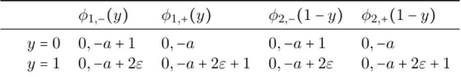
ρ^±₁, ρ^±₂ Exponents of system (2.4) and (2.5) at y=0,1 21 K,K˜ Second order elements of U(sl₁) used to capture the

eigenvalue problem of AQRM

22

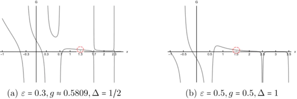
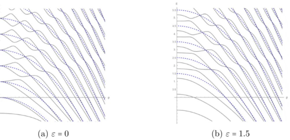
G_ε(x;g,∆) G-function of the AQRM 24

P_k^(N,ε)(x, y) Constraint polynomial of the AQRM 29

c^(ε)_k c^(ε)_k =k(k+ε) 35

λ_k λ_k=k(k−1)(N−k+1) 35

(a)ⁿ Pochhammer symbol 29

tridiag⎡⎢

⎢⎢⎢⎣

a_i b_i ci

⎤⎥⎥⎥

⎥⎦^1≤i≤n Tridiagonal matrix with main diagonal{a}ⁱ, upper diagonal {b}ⁱ and lower diagonal{c}ⁱ.

29 e_i The i-th basis vector of the standard basis of R^k 36 Tε^(N)(g,∆) Constraint function for exceptional non-Juddian

eigenvalues of AQRM

56 Gε(x;g,∆) GeneralizedG-function of the AQRM 64

K

^∞^k=1⁽^abⁿn) The continued fraction with partial numeratorsanand partial denominators b_n

70 Q^(N,)_k (x, y) OPS associated to constraint polynomials 70

2F1(a, b;c;s) Gauss hypergeometric function 71

1F₁(a;b;s) Confluent hypergeometric function 71

2F2(a, b;c, d;s) Generalized hypergeometric function 73

γ(s, x) Incomplete gamma function 73

(10)

Introduction

Thequantum Rabi model(QRM), originally described in [24], is the fully quantized version of the semi-classical model defined in [47] by Isidor Isaac Rabi in 1936 to describe the effect of a rapidly varying weak magnetic field on an oriented atom possessing nuclear spin. The QRM is one of the basic models in quantum optics, as it describes the simplest interaction between a two-level atom and a light field.

The Hamiltonian of the QRM is given by

H_Rabi=ωa^†a+g(a+a^†)σ_x+∆σ_z,

where σx, σz are the Pauli matrices, ω > 0 is the classical frequency of light field (modeled by a quantum harmonic oscillator), 2∆ > 0 is the energy difference of the two-level system andg>0 is the interaction strength between the two system.

Different combinations of the parameters of the model are classified intoparameter regimes according to the static and dynamic properties of its energy levels and solutions (see [45] for a discussion on the different parameter regimes).

For a long time, experimental realizations of the QRM achieved parameters regimes in which the dynamic and static properties could be approximated successfully by theJaynes-Cummings model [24]. The Jaynes-Cummings model was long known to be exactly solvable, and its physical properties could be compared with the experimental results. However, recent development in experimental physics [37, 65]

have been able to realize parameter regimes (for instance the nonperturbative ultrastrong coupling and the deep strong coupling regimes) were the Jaynes-Cummings model (or other similar approximations) is no longer suitable to describe its physical properties. These developments, along with the prospect of applications to areas such as quantum information technologies (see [18, 50, 65]) have made the study the properties of the QRM and its spectrum a priority in physics.

Despite the simplicity of its definition, using only raising and lowering operators of a quantum harmonic oscillator and Pauli matrices, only a set of degenerate eigenvalues, known asJuddian eigenvalues[25], was explicitly known for a long time. It was not until 2011, when Daniel Braak, exploiting theZ/2Z-symmetry found in the Hamiltonian, was able to construct analytic solutions and describe the eigenvalues (with the exception of a (possibly finite) set ofexceptional eigenvalues) as the zeros of a transcendental function, called G-function [5]. Since then, several extensions and generalizations of the QRM have been solved by using techniques derived of Braak’s work (see e.g. [7, 13]).

The asymmetric quantum Rabi model (AQRM) is one of these generalizations.

The Hamiltonian of the AQRM is obtained by introducing a non-trivial interaction term that breaks theZ/2Z-symmetry in the Hamiltonian of the QRM. Concretely, its Hamiltonian is given by

H_Rabi^ε =ωa^†a+∆σz+gσx(a^†+a) +εσx,

(11)

withε∈R. The absence of theZ/2Z-symmetry makes the presence of degeneracies in this model highly nontrivial, in particular there appears to be no way to define invariant subspaces (called parity subspaces in the case of the QRM) whose solutions constitute degeneracies (or crossings). Concretely, by using the symmetry found in the QRM, it is seen that H_Rabi = H+∆⊕H−∆ for Hamiltonians H±∆ acting on appropiate subspaces of the Hilbert space in which H_Rabi acts. Degeneracies are then found to appear between one eigenvalue of H_+∆ and one eigenvalue of H_−∆. Such a decomposition is not known for the AQRM.

Strikingly, degenerate states were discovered in numerical experiments for the caseε= ¹2 by Li and Batchelor in [33]. Later, Masato Wakayama in [63] conjectured the existence of degenerate states for the general half-integer ε case in terms of divisibility of constraint polynomials and proved the conjecture for the caseε= ¹₂. The conjecture was recently proved affirmatively for the general case by Kazufumi Kimoto, Masato Wakayama and the author in [27]. The presence of degenerate solutions for half-integer parameter actually hints at the possibility of a hidden symmetry in the AQRM, as it has been discussed in [63, 53].

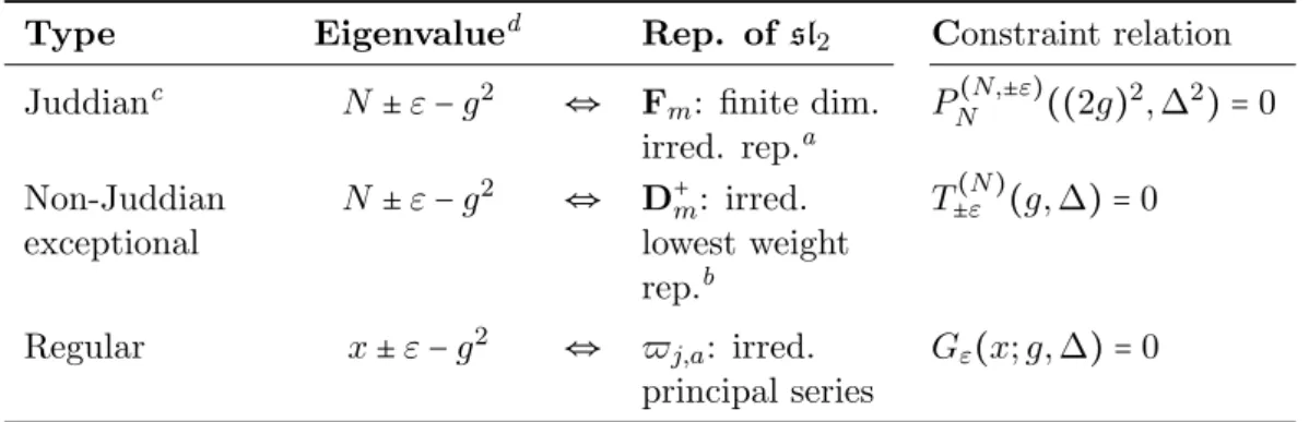
As in the case of the QRM, there is aG-functionGε(x;g,∆)for the AQRM that determines the regular eigenvalues, that is, all the eigenvalues with the exception of a set of exceptional eigenvalues of the form λ= N±ε−g², with N ∈ Z≥0. The exceptional eigenvalues are further classified into two types, Juddian eigenvalues, when the solutions of the eigenvalue problem in the Segal-Bargmann spaceH^B can be represented by a polynomial, that is, is a quasi-exact solution, or non-Juddian exceptional eigenvalues when this is not the case. The presence of the Juddian eigenvalueλ=N±ε−g² is equivalent to the constraint relation

P_N^(N,±ε)((2g)²,∆²) =0,

whereP_N^(N,±ε)(x, y) is a polynomial of degree N, called constraint polynomial (see [33] and [31] for the case of the QRM). As it is clear from the definitions, a necessary condition for two exceptional eigenvalues λ₁ =N+ε−g² and λ₂ =M−ε−g² with N, M∈Z≥0 and N /=M, to be equal is that

ε= M−N 2 = `

2 ∈ 1 2Z,

that is,ε must be half-integer. Since the regular eigenvalues are known to be non- degenerate (see [5] and Section 2.6 below), this is actually a necessary condition for the AQRM to have degenerate eigenvalues. Furthermore, as we show in Corollary 4.1.4, there are no degeneracies consisting of a Juddian and a non-Juddian exceptional solution. Therefore, any possible degeneracy in the spectrum of the AQRM must consist of two Juddian solutions. In terms of constraint polynomials, this is equivalent to the simultaneous satisfaction of the two constraint relations

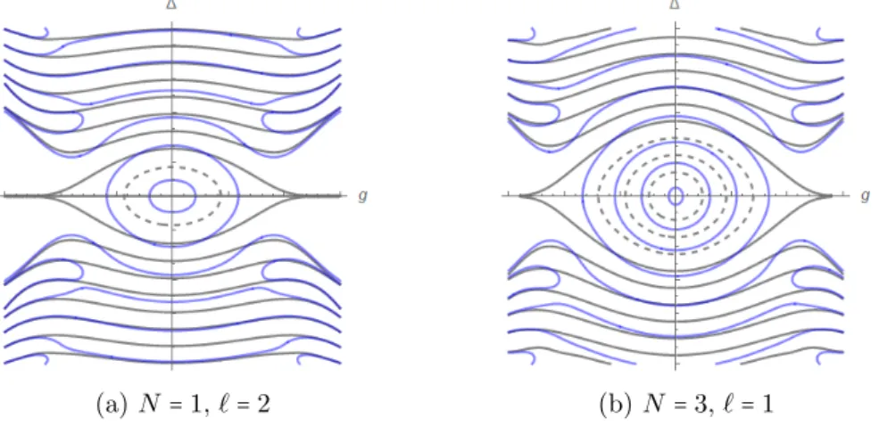
P_N^(N,`/2)((2g)²,∆²) =0=P_N^(N_+`^+`,−`/2)((2g)²,∆²), (1) whereN ∈Z≥0 and`≥0 (for`<0 it is enough to switch the roles ofN andM in the discussion above). In addition, if all the roots of the polynomial on the left-hand side of (1) are roots of the polynomial in the right-hand side, and viceversa, then all Juddian solutionsλ=N+`/2−g² must be degenerate. Since the polynomials on

(12)

both sides are of different degrees, except in the case of `=0 (i.e. the QRM), the relation (1) is nontrivial.

Following this argumentation, the conjecture given by Masato Wakayama in [63]

is that the divisibility relation

P_N^(N_+`^+`,−`/2)(x, y) =A_N^` (x, y)P_N^(N,`/2)(x, y),

holds for N, `∈ Z≥0 and that the polynomials A^`_N(x, y) have no positive roots for x, y>0. In other words, that any Juddian eigenvalue of the AQRM is degenerate when the parameterε is half-integer. The proof of the conjecture in [27] was done by studying certain determinant expressions satisfied by the constraint polynomials.

The proof presented in this thesis is a generalization of the said proof, in fact, we prove a stronger conjecture, also proposed in [63] (see Section 2.9).

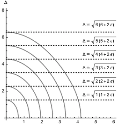
Another important question is to determine whether exceptional solutions do, in fact, appear in the spectrum for given parameters g,∆>0. A result of Li and Batchelor, presented in [33], gives a lower bound on the number of roots of the constraint polynomials when the parameter ∆ is in certain intervals. In Section 3.5 we prove a stronger formulation of the result, giving the exact number of solutions for the same intervals. This result suffices for the case of Juddian eigenvalues.

For non-Juddian exceptional eigenvalues, we define a transcendental constraint T-function Tε^(N⁾(g,∆) such that the equation

T_ε^(N)(g,∆) =0

is equivalent to the presence of the non-Juddian exceptional eigenvalueλ=N+ε− g². Aside from providing conditions for the existence of non-Juddian exceptional solutions, these T-functions appear, along with the constraint polynomials, in the expression of the residues of theG-function of the AQRM. By using this, we define a generalizedG-functionG^ε(x;g,∆) whose zeros determine the complete spectrum of the AQRM. In other words, it is essentially (up to a nonvanishing entire factor) the spectral determinant for the Hamiltonian of the AQRM.

The purpose of this thesis is to give a complete overview of the spectrum of the AQRM, including the complete characterization of the degeneracies in its spectrum.

The thesis is intended to be a mostly self-contained exposition, however for a number of results we refer the reader to the original sources.

We begin, in Chapter 1 by giving an overview of the quantum harmonic oscillator and its raisinga^†and loweringaoperators and theirL²(R)and Segal-Bargmann space H^B space realizations. Furthermore, we give basic overview of the representation theory of the Lie algebrasl₂ and its irreducible representations.

In Chapter 2, we present a short historical review of the main research done on the QRM starting from its definition. In Section 2.2, we give a tour of the Hamiltonians of several models of quantum optics that describe the interaction between light and matter. Several of these models are generalizations of the QRM.

In Section 2.3, by considering the realization as a second order pseudo-differential operator acting onL²(R)⊗C²we give some of general properties of the Hamiltonian of the AQRM and its spectrum, the most important being that the spectrum consist only of the discrete set of eigenvalues. Next, in Section 2.4 we study the realization of eigenvalue problem of the Hamiltonian of the AQRM in the Segal-Bargmann

(13)

space and reduce it to a system of two linear differential equations, equivalent to a confluent Heun differential equation. Moreover, this system is captured by elements of the universal enveloping algebra of sl₂. In Section 2.5, we describe the classification of the eigenvalues of the AQRM into regular eigenvalues, further discussed in Section 2.6, and exceptional eigenvalues, discussed in 2.7, according to the Frobenius solutions of the system of linear differential equations of confluent Heun type. In Section 2.8, we describe how the constraint polynomials are related to the coefficients of the solutions of the differential equation system, in particular we prove the equivalence of the constraint relation with the presence of Juddian eigenvalues. In Section 2.9, we discuss the conjectures on constraint polynomials that gave the motivation for this research.

In Chapter 3, we study the constraint polynomials and its mathematical properties. Above all, we see how the “divisibility” of the conjectures follows from certain determinant expressions related to their definition by three-term recurrence relations. The positivity follows as well by the properties of the eigenvalues of the matrices involved in said determinant expressions. The conjectures are finally proved in Section 3.3. In Section 3.5, we prove the already mentioned result on the number of positive roots of constraint polynomials when one of the variables is in a given interval. In Section 3.6 we give some explicit formulas for constraint polynomials that can be used to study the constraint polynomials from the combinatorial point view.

In Chapter 4 we complete the picture of the spectrum of the AQRM, by describing the degeneracy structure using the results of the previous chapters. Notably, in Section 4.1 we characterize the degeneracy of the exceptional spectrum of the AQRM, this being sufficient to describe the degeneracy structure in the general case. In Section 4.2, we derive the aforementioned constraint T-function, that, along with the constraint polynomials, is used to study the residues of the poles of theG-function in Section 4.3. In Section 4.4 we define the generalized G-function and prove that its zeros determine the full spectrum of the AQRM. Finally, in Sec- tion 4.5 we show that exceptional solutions correspond to eigenvectors in irreducible sl₂-modules in the sl₂-picture of the eigenvalue problem of the AQRM.

As an addendum to the study of the spectrum of the AQRM, in Chapter 5 we present certain continued fraction expansions for powers of the Napier constant (or Euler’s number)eⁿ, withn∈Z≥0with good convergence properties. These continued fraction expansions appeared during the study of certain orthogonal polynomial families related to the constraint polynomials. This study is intended to give an example of the rich mathematical structure appearing in the study of the AQRM and its spectrum.

The year 2016 marked the 80 anniversary of the publication of the original paper by Rabi describing his original model, see [4] for a review of the QRM commemo- rating the occasion. Even after 80 years and a large amount of research (a search on arXiv.org shows more than 100 entries for quantum Rabi model and related topics since 2011), the list of mysteries and open questions concerning the quantum Rabi model is very large and is still growing. A short discussion on certain open problems is given in Chapter 6 with the hope that it motivates further research in the quantum Rabi model.

As a disclaimer, we note that some of the results of Section 2.8 and Chap-

(14)

ters 3 and 4 are (or are generalizations of) results published in [48], with Masato Wakayama, and [27], with Kazufumi Kimoto and Masato Wakayama. The results of Chapter 5 consist of previously unpublished work.

(15)

1. Preliminaries

The purpose of this chapter is to give a brief introduction of the tools and concepts to be used later in the study of the spectrum of the asymmetric quantum Rabi model.

First, we give an overview of the theory of the quantum harmonic oscillator, a model of quantum physics that is used to describe more complicated physical phenomena. Next, we introduce the Segal-Bargmann space, a Hilbert space of entire functions in which the realization of the raising and lowering operators of the harmonic oscillator have a particularly simple expression. In this Hilbert space, the eigenvalue problem of the quantum Rabi model reduces to a system of ordinary linear equations of confluent Heun type. As it is well-known, differential equations can be realized by elements of U (sl₂), the universal enveloping algebra of sl₂ via certain representations. For this reason, in the final section we introduce the basic theory ofsl₂ representations that we use in later chapters.

1.1 The quantum harmonic oscillator

The quantum harmonic oscillator is one the simplest models in quantum mechanics.

Its importance lies in that it has simple analytic solutions and that a good number of physical phenomena is modeled using coupled harmonic oscillators. For instance, the quantum Rabi models studied in this thesis are defined in terms of the the raising and lowering operatorsa anda^† that appear in the quantum harmonic oscillator.

LetHbe a Hilbert space. Consider self-adjoint operatorsX and P acting onH satisfying the conmutation relation

[X, P] =i̵h1,

and the hypothesis of the Stone-von Neumann theorem (see [17], Chapter 14). The constanth̵ =1.054×10⁻²⁷ erg⋅s=1.054×10⁻³⁴ J⋅s, is the reduced Planck constant.

The Hamiltonian of the one-dimensional quantum harmonic oscillator (QHO), or linear oscillator, is given by

H= 1 2(P²

m +kX²),

wherem, k>0. The constant m is interpreted as the mass of the particle.

Introducing the constantω, calledthe classical frequencyof the oscillator, given by

ω=

√k m, the HamiltonianH is written as

H= 1

2m(P²+ (mωX)²).

(16)

1.1. The quantum harmonic oscillator Next, we introduce the raising operator a^† and the lowering operator a, by the formulas

a^†= mωX−iP

√2̵hmω , a= mωX+iP

√2̵hmω .

The operatora^† is also calledcreation operator, and correspondingly, the operator ais called annihilation operator. The operatora^† is the adjoint of a, justifying the notation.

By direct computation, we observe that [a, a^†] =1, where1 is the identity operator.

The Hamiltonian H is written in terms of the operators aand a^† as H= ̵hω(a^†a+1

21),

and therefore the study of the spectrum of the QHO is reduced to the study of the spectrum of the self-adjoint operatora^†a. The spectrum of the operator a^†a, and therefore of the QHO, can be described explicitly. We recall the results here and refer the reader to [17, 58, 64], for a more detailed discussion.

The following result justifies the name raising and lowering for the operatorsa^† anda, its proof is immediate from the commutation relation above.

Proposition 1.1.1. Let φbe an eigenfunction ofa^†awith eigenvalue λ∈R. Then, a^†a(aφ) = (λ−1)φ

a^†a(a^†φ) = (λ+1)φ.

Since a and a^† are adjoint operators, any eigenvalue λ of a^†a is non-negative, and thus by the proposition above ifφis an eigenfunction of a^†athere must beφ0, a ground state, with a^†aφ₀ = 0 and φ= (a^†)ⁿφ₀ for a non-negative integer n. In particular,λitself is a non-negative integer.

Proposition 1.1.2. If φ₀ is a unit vector withaφ₀=0, then for n≥0, define φ_n= (a^†)ⁿφ₀.

The following relations hold forn≥0, a^†aφn=nφn

aφn+1= (n+1)φn. Furthermore, the family{φ_n}n≥0 is orthogonal.

Depending on the choice of Hilbert space H, it may be the case that there are multiple independent ground states, for example in the Hilbert space L²(R) ⊗ C², equipped with the inner-product inherited from L²(R), there are two linearly independent ground states.

(17)

1.2. The Segal-Bargmann space Finally, we make some considerations for the case of H = L²(R). In this realization, the eigenvectors are given explicitly by the Hermite functions. Setting, for simplicity, ̵h =m =ω = 1, we see that the position operator is realized by the multiplication operator

X=x,

and the momentum operator is realized by the differentiation operator P = −i d

dx.

The raising and lowering operators are then given by a^†= 1

√2(x− d

dx), a= 1

√2(x+ d dx),

and the equation aφ0 = 0 is an ordinary differential equation of order one with general solution

φ0(x) =Ce^−x²^/2,

and where the normalization condition gives immediatelyC=√ π.

Proposition 1.1.3. The ground state φ0(x) of a^†ais given by φ₀(x) =√

πe^−x²^/2, and the “excited states”φn(x) are given by

φn(x) =Hn(x)φ0(x),

where H_n(x) is then-th Hermite polynomial, defined by the equation dⁿ

dxⁿ(e⁻¹²^x²) = (−1)ⁿe⁻¹²^x²Hn(x).

Furthermore, the family{φ_n(x)}≥0 is an orthonormal basis of H =L²(R). Therefore, in theH =L²(R) realization, the spectrum of the QHO is

Spec(H) = {̵hω(n+1

2) ∶n∈Z≥0},

in particular, the eigenvalues (energy levels) of the QHO differ by integer multiples of the quantity ̵hω. In this thesis, we assume h̵ =1 in the sequel, without loss of generality, to simplify the discussion.

1.2 The Segal-Bargmann space

In this section we give an overview of the Segal-Bargmann space H^B (cf. [2]), also known as Bargmann space, Bargmann Fock space or Fock space. It is often used to study the spectrum of quantum systems, including the quantum Rabi model and related models. The spaceH^B was originally defined for holomorphic functions in

(18)

1.2. The Segal-Bargmann space Cⁿ, but it suffices to consider the one dimensional case for the applications presented in this work. We follow the description given in [17].

Let V(C) be the space of holomorphic functions f ∶C→C. An inner-product inV(C) is defined for f, g∈ V(C)by

(f, g)^B= ∫

C

f(z)g(z)dµ(z) (1.1) where the measuredµ(z) is given bydµ(z) = ¹_πe^−∣z∣²dxdy forz=x+iy, anddxdy is the Lebesgue measure inC≃R².

The Segal-Bargmann space H^B is the space of entire functions f ∶ C → C in V(C) satisfying

∥f∥^B= (f, f)^1/2B = (∫

C∣f(z)∣²dµ(z))^1/2 < ∞.

Theorem 1.2.1([17] Proposition 14.15). The Segal-Bargmann spaceH^B is a complete Hilbert space with respect to the inner product(⋅,⋅)^B given in (1.1). In addition, the set of (holomorphic) polynomials forms a dense subspace ofH^B.

An important property of the space H^B (see [8]) for the study of the spectrum of the quantum Rabi model is that it contains entire functions having asymptotic expansion of the form

e^α¹^zz^−α⁰(c₀+c₁z⁻¹+c₂z⁻²+ ⋯), (1.2) as z → ∞. A particular case is that of normal solutions of differential equations having an unramified irregular singular point of rank 2 at infinity. This fact is important for the study of the eigensolutions of asymmetric quantum Rabi model.

The multiplication operator Z = z and differentiation operator Y = ∂_z = _dz^d acting onH^B satisfy the commutation relation

[Y, Z] =1,

in other words, they satisfy the same commutation relations as the raising and lowering operators of Section 1.1. In fact, if f, g are (holomorphic) polynomials, then it holds that

∫C(f(z)∂zGdµ(z) = ∫

C

zf(z)g(z)dµ(z). In general, we have the following result.

Proposition 1.2.2. The multiplication operator Z =z is the adjoint of the differentiation operatorY =∂z in H^B.

In light of the Theorem 1.2.1 and Proposition 1.2.2, the multiplication and differentiation operators are (formally) realizations of the raising and lowering operators a^† and a.

Next, define the operators

A= 1

√2(Z+Y) B= i

√2(Z−Y).

(19)

1.3. Representation theory ofsl₂ The operators Aand B are self-adjoint and satisfy the hypothesis of the Stone- von Neumann theorem, and thus there is a unitary mapU ∶ H^B→L²(R) satisfying

U eîtAU⁻¹=eîtX U eîtBU⁻¹=eîtP

whereX and P are the usual position and momentum operators acting onL²(R). The inverse of the map U can be computed explicitly and is called the Segal- Bargmann transform (See [17] Theorem 14.18). This argument shows that the multiplicationZ and differentiation operatorY are indeed equivalent to the raising and lowering operators introduced in Section 1.1 for the Hilbert spaceL²(R).

For the study of the spectrum of operators, the Segal-Bargmann H^B has the advantage that the realization the raising and lowering operators is of lower degree (as a differential operator) than in the standard L²(R) realization. In addition, elements ofH^B are functions and not equivalence classes of functions like inL²(R). We refer the reader to [2, 17] for a more detailed description of the Segal-Bargmann space and to [52] for more applications to the eigenvalue problem of quantum systems.

1.3 Representation theory of sl

2

In this section we recall some basic representation theory ofsl₂(R)used in the next chapter to describe thesl₂(R)-picture of the eigenvalue problem of the AQRM. The reader is directed to [20, 32, 57] for the general theory ofsl₂-representations.

LetM2(R) the algebra of real 2×2 matrices andGL2(R) be the general linear groupof real matrices, that is, the (multiplicative) subgroup ofM₂(R)consisting of invertible real matrices. Thespecial linear group SL₂(R) is the closed subgroup of GL2(R)given by

SL₂(R) = {M ∈GL₂(R) ∣det(M) =1}.

From general theory, we know thatSL2(R) is a non-compact and semisimple con- nected Lie group. The Lie algebra of SL₂(R), denoted by sl₂, or sl₂(R), is given by

sl₂= {M∈M2(R) ∣ tr(M) =0},

is asimpleLie algebra. Denote byg_Cthe complexification of the Lie algebrag, then it is not difficult to verify that(sl₂)_Cissl₂(C), the Lie algebra ofSL2(C)(c.f. [57]).

In Section 2.4, we capture the eigenvalue problem of the asymmetric quantum Rabi model, reduced to a system of two linear equations of Heun type, by an element of the universal enveloping algebraU(sl₂). Recall that ifg is a Lie algebra, define T0(g) =C,T⁽ⁿ⁾(g) =g^⊗n, with

g^⊗n=g⊗g⊗ ⋯ ⊗g

´¹¹¹¹¹¹¹¹¹¹¹¹¹¹¹¹¹¹¹¹¹¹¹¹¹¹¹¹¹¹¹¸¹¹¹¹¹¹¹¹¹¹¹¹¹¹¹¹¹¹¹¹¹¹¹¹¹¹¹¹¹¹¹¶

n

,

then, the tensor algebraT(g) is given by T(g) =⊕^∞

n=0

T_n(g).

(20)

1.3. Representation theory ofsl₂ LetJ be the ideal ofT(g_C) generated by the elements

[X, Y] − (X⊗Y −Y ⊗X)

withX, Y ∈g_C, then theuniversal enveloping algebraof g is given by U(g) =T(g_C)/J.

The universal property ofU(g) is that every representation of g extends to a representation ofU(g)(see [20], Section 1.3).

A set ofstandard generatorsofsl₂ is given by the matricesH, E andF ofsl₂(R) defined as

H= [1 0

0 −1], E= [0 1

0 0], F = [0 0 1 0]. These generators satisfy the commutation relations

[H, E] =2E, [H, F] = −2F, [E, F] =H.

Next, let us introduce a representation of sl₂, depending on a parameter a∈C, which is used to capture the confluent Heun differential equations in Section 2.4.

The reader is directed to [63] for an extended discussion of this representation. Let a∈C and define the action $_a of sl₂ on the vector spaces V₁ ∶=y⁻¹⁴C[y, y⁻¹] and V2∶=y¹⁴C[y, y⁻¹] by

$a(H) ∶=2y∂y+1

2, $a(E) ∶=y²∂y+1 2(a+1

2)y, $a(F) ∶= −∂y+1 2(a−1

2)y⁻¹ with ∂_y ∶= _dy^d. It is not difficult to verify that this defines infinite dimensional representations of sl₂. Write $_j,a ∶=$_a∣Vj and put e_1,n ∶=yⁿ⁻¹⁴ and e_2,n ∶=yⁿ⁺¹⁴. Then we have

⎧⎪⎪⎪⎪⎪⎪⎪

⎨⎪⎪⎪⎪⎪⎪⎪

⎩

$1,a(H)e1,n=2ne1,n,

$1,a(E)e1,n= (n+a

2)e1,n+1,

$_1,a(F)e_1,n= ( −n+a

2)e_1,n−1,

⎧⎪⎪⎪⎪⎪⎪⎪⎪

⎨⎪⎪⎪⎪⎪⎪⎪⎪

⎩

$_2,a(H)e_2,n= (2n+1)e_2,n,

$2,a(E)e2,n= (n+a+1

2 )e2,n+1,

$2,a(F)e2,n= ( −n+a−1

2 )e2,n−1. Whena/∈2Z(resp. a/∈2Z−1) the representation($_1,a,V₁)(resp. ($_2,a,V₂)) is an irreducible representation, calledprincipal series. Note that there is an equivalence between$j,a and $j,2−a under the same condition.

For a non-negative integerm, define subspacesD^±_2m,F_2m−1ofV_1,2m(=V₁), and D^±_2m+1,F2m ofV2,2m+1(=V2) respectively by

D^±_2m∶= ⊕

n≥m

C⋅e1,±n, F2m−1∶= ⊕

−m+1≤n≤m−1

C⋅e1,n, D⁻_2m+1∶= ⊕

n≥m+1

C⋅e_2,−n, D⁺_2m+1∶= ⊕

n≥mC⋅e_2,n, F_2m∶= ⊕

−m≤n≤m−1

C⋅e_2,n. The spaces D^±_2m (resp. D^±_2m+1) are invariant under the action $_1,2m(X), (resp.

$2,2m+1(X)), (X ∈sl₂), and define irreducible representations (having lowest and

(21)

1.3. Representation theory ofsl₂ highest weight vector respectively) known to be equivalent to (holomorphic and anti- holomorphic)discrete seriesform>0 ofsl₂(R). The irreducible representationD^±₁ are the(infinitesimal version of ) limit of discrete series ofsl₂(R)(see e.g. [20, 32]).

Moreover, the finite dimensional spaceFm (dim_CFm=m), is invariant and defines irreducible representation of sl₂ for a= 2−2m when j = 1 and a = 1−2m when j=2, respectively. We remark here that the finite dimensional representations F_m are not unitarizable.

The following result describes the irreducible decompositions of($a,Vj,a) (a= m≡j−1 mod 2)form∈Z≥0andj=1,2. In particular, it gives the relation between the finite representationsF_m and the invariant submodules D^±_m.

Lemma 1.3.1. Let m∈Z≥0.

1. The subspaces D^±_2m are irreducible submodules of V_1,2m under the action

$1,2m and F2m−1 is an irreducible submodule of V1,2−2m under $1,2−2m. In the former case, the finite dimensional irreducible representation F2m−1 can be obtained as the subquotient as V_1,2m/D⁻_2m⊕D⁺_2m ≅ F_2m−1. In the latter case, the discrete series D^±_2m can be realized as the irreducible components of the subquotient representation as V1,2−2m/F2m−1≅D⁻_2m⊕D⁺_2m.

2. The subspaces D^±_2m+1 are irreducible submodule of V2,2m+1 under the action

$2,2m+1 and F2m is an irreducible submodule of V2,1−2m under $2,1−2m. In the former case, the finite dimensional irreducible representation F_2m can be obtained as the subquotient as V2,2m+1/D⁻_2m+1⊕D⁺_2m+1 ≅ F2m, while in the latter case, the discrete series D^±_2m+1 can be realized as the irreducible components of the subquotient representation as V_2,1−2m/F_2m≅D⁻_2m+1⊕D⁺_2m+1. 3. The space V_2,1 is decomposed as the irreducible sum: V_2,1=D⁻₁ ⊕D⁺₁. Moreover, the spaces of irreducible submodulesD^±_m(⊂Vj,m),Fm(⊂Vj,1−m) and the direct sumD⁺_m⊕D⁻_m(⊂V_j,m) above are the only non-trivial invariant subspaces of Vj,m for j=1 (resp. j=2) when m is even (resp. odd) under the action ofU(sl₂), the universal enveloping algebra of sl₂.

In Section 4.5, we make use of the isomorphism described in the proposition above to describe how certain solutions of the eigenvalue problem of the quantum Rabi model determine elements in irreducible submodules ofsl₂(R).

(22)

2. The asymmetric quantum Rabi model

This chapter is an introduction to the study of the quantum Rabi model and its generalization, the asymmetric quantum Rabi model.

First, in Section 2.1 we give a short historical note on the research done on the quantum Rabi model and its spectrum, including experimental realizations. In Section 2.2 we give a tour of the Hamiltonians of various models describing the interaction of light and matter, including the quantum Rabi model and different generalizations. After that, in Section 2.3 we focus on the asymmetric quantum Rabi model and give some general properties of its Hamiltonian when considered as an operator acting inL²(R) ⊗C².

In Section 2.4, by using the Segal-Bargmann H^B space realization we see that the eigenvalue problem of the AQRM reduces to a set of two linear ordinary differential equations of confluent Heun type and how they can be captured in the sl₂-representation picture. Next, in Section 2.5, we give the classification of the spectrum of the AQRM according to the type of the solutions of the aforementioned system. In particular, there is a regular spectrum governed by the zeros of a G-function, described in Section 2.6. The remaining eigenvalues of the AQRM are called exceptional, these appear from certain solutions of the differential equation system where the difference of the exponents are integer. These solutions are studied in Section 2.7, where we see that there can be polynomial solutions, called Juddian solutions, and non-polynomial, called non-Juddian exceptional solutions.

The Juddian solutions are determined by the roots of certain polynomials, called constraint polynomials. In Section 2.8, we see how these polynomials are related to the coefficients of the solutions of the differential equation system. Finally, in Section 2.9 we describe, in terms of constraint polynomials, the conjectures on the degeneracy of the Juddian solutions of the AQRM, proposed by Masato Wakayama in [63]. In Chapter 3 we prove these conjectures, and in Chapter 4 complete the degeneracy picture of the asymmetric quantum Rabi model.

2.1 A brief history of the quantum Rabi model

In this section we give a short historical review on the research on the QRM relevant to the studies in the present thesis. It is important to note that due to the amount of research done on the QRM, any such list is necessarily incomplete. For more information on the experimental realizations and parameter regimes of the QRM, we refer the reader to [45, 51] (see also the discussion on Section 6.3)

In 1936, Isidor Isaac Rabi introduced in [47] a model to discuss the effect of a rapidly varying weak magnetic field on an oriented atom possessing nuclear spin.

(23)

2.1. A brief history of the quantum Rabi model This model is the semi-classical version of the model which is now known as the quantum Rabi model. In 1944, Rabi would go on to receive the Nobel Prize in Physics for the discovery of nuclear magnetic resonances.

In 1963, E.T. Jaynes and F.W. Cummings considered in [24] the fully quantized version of the quantum Rabi model for the case where the rotating-wave approximation applies, that is, were the model now known as the the Jaynes-Cummings model successfully approximates the QRM.

In 1979, Judd described in [25] the presence of quasi-exact solutions which are now known as Juddian eigenvalues.

In 1987, Ku´s showed in [31] the degeneracy of the Juddian eigenvalues and proved that there are at least n−k degenerate Juddian points for each value of n for ∆/ω satisfying k<∆/ω<k+1.

In 2007, Gleyzes, Kuhr, Guerlin, Bernu, Del`eglise, Hoff, Brune, Raimond and Haroche in [16] realized the QRM experimentally in thestrong coupling regimeusing a single atom in the context of cavity in microwave cavity quantum electrodynamics experiments. In this regime, the model can be successfully approximated by the Jaynes-Cummings model.

In 2009, Anappara, De Liberato, Tredicucci, Ciuti, Biasiol, Sorba and Beltram in [1] reported signatures of the QRM of theperturbative ultrastrong coupling regime in a quantum-well intersubband microcavity. In this case, the Jaynes-Cummings model is not suitable to approximate the properties of the energy levels of the QRM, however it can still be approximated by the Bloch-Siegert Hamiltonian.

In 2011, Daniel Braak constructed in [3] analytical solutions of the QRM and gave conditions for existence by showing the existence of a transcendental function whose zeros exactly describe the eigenvalues of the QRM. He also conjectured that the spacing between two consecutive eigenvalues of the QRM is always less than or equal to 2 and gave a (conjectural) description on the number of eigenvalues in intervals[n, n+1)forn∈Z≥0. In the same paper, he defined the AQRM (under the name of generalized QRM) and extended his results on solvability to it.

In 2012, M. Hirokawa and F. Hiroshima proved in [19] that the ground state of the quantum Rabi model is non-degenerate.

In 2012, Chen, Wang, He, Liu and Wang reformulated Braak’s result in [9] using the Bogoliubov transform avoiding the use of Segal-Bargmann space methods.

In 2013, Zhong, Xie, Batchelor and Lee showed in [67] the existence of analytic solutions using confluent Heun functions. This method is equivalent to the G- function approach.

In 2013, A.J. Maciejewski and M. Przybylska and T. Stachowiak showed in [36]

the existence of non-Juddian exceptional eigenvalues numerically and gave conditions for their presence in terms of the confluent Heun functions. The existence of non-Juddian exceptional solutions has not been considered before the publication of this work.

In 2014, Masato Wakayama proved in [61] (see also [62]) that the eigenvalue problem of the quantum Rabi model can be captured by a second order element R ∈ U(sl₂) via a confluent process. The element R ∈ U(sl₂) is associated to the eigenvalue problem of the non-commutative harmonic oscillator via certain representation, the reader is refered also to [39] for more information.

(24)

2.2. Matter and light interaction models In 2014, M. Wakayama and T. Yamasaki showed in [60] the existence of a second order elementK∈ U(sl₂) that realizes the eigenvalue problem of the quantum Rabi model via a representation (described in Section 1.3). This is sl₂-representation picture of the QRM.

In 2014, Maissen, Scalari, Valmorra, Beck, Fais, Cibella, Leoni, Reichl, Char- pentier and Wegscheider in [37] successfully realized experimentally the QRM in thenonperturbartive ultrastrong coupling regime using metallic and superconduct- ing complementary split-ring resonators coupled to the cyclotron transition of two- dimensional electron gases. In this coupling regime, the Jaynes-Cummings model, or other approximations like the Bloch-Siegert Hamiltonian, are not appropriate to study the energy levels of the QRM.

In 2015, Li and Batchelor in [33] made the striking numerically discovery of degenerate Juddian points in the spectrum of AQRM for the parameter ε = ¹2. Furthermore, they explicitly defined the constraint polynomials for the Juddian solutions and extended some of Ku´s results on constraint polynomials (see Section 3.5 for discussion on this result).

In 2015, Pedernales, Lizuain, Felicetti, Romero, Lamata and Solano proposed in [44] a method to simulate the quantum Rabi model in all parameter regimes by means of detuned bichromatic sideband excitations of a single trapped ion. In particular, this proposal permits the simulation of the QRM in the ultrastrong and deep strong couplings regimes using current setups.

In 2016, Shingo Sugiyama proved in [55] that the spectral zeta function of the QRM

ζ_H_Rabi(s) = ∑

λ∈Spec(HRabi)

1 λ^s

can be extended meromorphically to the complex plane with a single pole ats=1.

In addition, he showed that

N_H(T) ∼2T

asT → ∞, whereN_H(T) is the number of eigenvalues smaller thanT ∈R. Asymp- totics for the spectrum of the type N_H(T) ∼ 2T are in general called Weyl laws.

This result supports Braak’s conjecture on the distribution of eigenvalues of the QRM.

In 2017, Masato Wakayama proved in [63] the existence of degenerate Juddian states for the case ε = ¹₂ and conjectured the result for general half-integer ε =

`/2∈ ¹₂Zin terms of divisibility of constraint polynomials. In addition, he described how the regular solutions and Juddian solutions can be captured in elements of irreducible representations in thesl₂-representation picture of the AQRM.

In 2017, Yoshihara, Fuse, Ashhab, Kakuyanagi, Saito and Semba in [65] successfully achieved thedeep strong coupling regime experimentally between a flux qubit and an LC oscillator. The authors expect that using this method the QRM can be realized in this parameter regime.

2.2 Matter and light interaction models

In this section we described several quantum models describing the interaction between light and matter. In general, the Hamiltonian of the models are given in the

(25)

2.2. Matter and light interaction models following general form

H= H_M

±atom

+H_L

°light

+ H_I

interaction terms°

where the HamiltonianHM corresponds to the two-level atom (or in general a two- level system), expressed by Pauli matrices σ_x,σ_y and σ_z

σx= (0 1

1 0), σy = (0 −i

i 0), σz= (1 0 0 −1),

the Hamiltonian HL corresponds to a photon field, described by the raising and lowering operators a^†, a of the QHO and, the interaction terms between the two systems, with Hamiltonian H_I. For a more detailed introduction to the study of these models, we refer the reader to [8].

The first category of models we describe are those where a number of two- level atoms are interacting with a single level photon field in a cavity. The main representative of these models is the quantum Rabi model, and the remaining models can be regarded as generalizations. As we discussed in Section 1.1, the Hamiltonians of these models are operators acting in a Hilbert spaceH⊗C^2M, whereHis a Hilbert space satisfying the hypothesis of the Stone-von Neumann theorem, with raising and lowering operatorsa^† and a, andM is the number of two-level atoms.

The quantum Rabi model(QRM) is often called the simplest model in quantum optics describing the interaction between light and matter. It describes the interaction between a two-level atom and a single level photon field. Its Hamiltonian H_Rabi is given by

HRabi=ωa^†a+g(a+a^†)σx+∆σz,

whereω>0 is the frequency of photon field in the cavity (essentially a QHO), 2∆>0 is the energy difference of the two-level system andg>0 is the interaction strength.

The QRM has aZ/2Z-symmetry, at the level of the Hamiltonian it amounts to the existence of a parity operator Π = −σz(−1)^a^†^a satisfying [Π, HRabi] = 0 and with eigenvaluesp= ±1 (c.f. [45]).

The main topic of study of this thesis, the asymmetric quantum Rabi model (AQRM), is a direct generalization of the QRM, defined by the Hamiltonian

H_Rabi^ε =H_Rabi+σ_x,

where∈R. The AQRM has been also referred to as generalized, biased or driven QRM (see, e.g. [5, 33, 45]). We remark that the QRM is considered to be an integrable model, but this is not the case for the AQRM. We direct the reader to [5] for the discussion on integrability of these models.

The presence of the termσxbreaks theZ/2Z-symmetry of the QRM, however a symmetry can be found by embedding the system into a larger system or by studying the Segal-Bargmann space realization of the system. We discuss this symmetry in Section 2.4 and Section 2.6 below.

The quantum Rabi model can be generalized for M two-level atoms interacting with a single level photon field with frequency ω >0. The Hamiltonian is defined

(26)

2.2. Matter and light interaction models as an operator acting on H ⊗C^2M and we denote by σx^(j), σz^(j) the Pauli matrices acting in thej-th atom. Concretely, the matrixσx^(j) is given by

σ_x^(j)=I2⊗ ⋯ ⊗I2⊗σx⊗I2⊗ ⋯ ⊗I2,

whereσ_x, the usual Pauli matrix, is at thej-th position. The matrixI₂ is the 2×2 identity matrix. The definition ofσz^j is completely analogous.

The Hamiltonian of the M-atom model H_{M a} is H_{M a}=ωa^†a+∑^M

i=1

∆_jσ^(j)_z +∑^M

j=1

g_j(a+a^†)σ_x^(j).

where the parameters(2∆1,2∆2, . . . ,2∆_M) ∈ (R^≥0)^M and(g1, g2, . . . , g_M) ∈ (R^≥0)^M are the difference in levels and coupling strengths between each of the two-level atoms and the photon field, respectively. Clearly, we haveH1a=H_Rabi⁰ .

Note that these models receive different names in accordance to certain conditions met by the parameters, for instance, if ∆_i= ¹₂∆>0 for all i=1,2, . . . , M the model is calledDicke model(see for instance [7] for the caseM =3).

We can also introduce theasymmetric M-atom model in the natural way. The Hamiltonian is given by

H_{M a}^ε =HM+∑^M

j=1

εjσ_x^(j),

for(ε1, ε2,⋯, ε_M) ∈R^M. Similarly to the one two-level atom model, the introduction of the additional term breaks the symmetries in the HamiltonianH_{M a}.

The following models are used to approximate the QRM and its generalizations described above. The main advantage of these models is that they are solvable and, therefore their spectrum is explicitly known.

The Jaynes-Cummings modelis the model with Hamiltonian H_JC=ωa^†a+g(σ⁺a+σ⁻a^†) +∆σ_z, whereσ^±= (σ_x±iσ_y)/2. Notice that the QRM can be written as

H_Rabi=ωa^†a+g(σ⁻a^†+σ⁺a) +g(σ⁺a^†+σ⁻a) +∆σz,

the term g(σ⁻a^†+σ⁺a) is called the rotating term and g(σ⁺a^†+σ⁻a) the counter- rotating term. From this point of view, the Jaynes-Cummings model is called the rotating wave approximation (RWA) of the QRM (see [24]) since it is obtained disregarding the counter rotating terms from the QRM. This model has a continuous U(1)-symmetry in contrast to the discrete Z/2Z-symmetry of the quantum Rabi model. The symmetry amounts to the existence of a conserved quantity (operator) N = a^†a+σ⁺σ⁻ with [HJC, N] = 0. Due to its symmetry the Jaynes-Cummings model is super-integrable and there is a explicit description of the eigenvalues of the Hamiltonian.

The generalization of the Jaynes-Cummings model forM two-level atoms is the Tavis-Cummings model(see [56]). Its Hamiltonian is given by

HT V =ωa^†a+∑^M

i=1

∆jσ_z^(j)+∑^M

j=1

g(σ^(j)+ a+σ−^(j)a^†),

(27)

2.3. General properties of the asymmetric quantum Rabi model whereσ±^(j) are defined in a manner analogous toσx^(j). The Tavis-Cummings model is integrable via Bethe ansatz methods and, like the Jaynes-Cummings model, has a precise description of its eigenvalues.

We conclude this section by listing certain models related to the QRM, but having a different structure in the Hamiltonian or in the spectral structure.

The two-photon quantum Rabi model, is the model with Hamiltonian given by HT P =ωa^†a+g((a)²+ (a^†)²)σx+∆σz.

The spectrum of this model behaves very differently than the QRM under the changes of parameters. In particular, it exhibits a spectral collapse phenomena (c.f.

[12]). Note that in the same way it is possible to formally defineM-photon quantum Rabi model, however it is known that these models are ill-defined for M ≥3.

The quantum Rabi-Stark model is a model describing an experiment where the single-level photon in a cavity is subject to two auxiliary laser beams. Its Hamilto- nian is given by

HRS =H_Rabi⁰ +γσza^†a.

Note that, compared to the QRM, the interaction includes the nonlinear terma^†a.

Its spectrum has been studied by adapting a method similar to the one used in the QRM (see [13]).

The last model that we describe in this section is not a generalization of the QRM. The non-commutative harmonic oscillator(NcHO), defined by Parmeggiani and Wakayama[42] in 2001, is the model with the Hamiltonian (acting onL²(R) ⊗ C²) given by

Q= [α 0 0 β] (−1

2 d² dx² +1

2x²) + [0 −1 1 0] (x d

dx+1 2),

for real parametersα, β. It is a formal model (it does not correspond to known physical phenomena) but a mysterious relation with the QRM has been found through a confluent process (c.f. [62]). The reader is refered to [43, 40] for an extensive introduction to the theory of the NcHO and to [41] for a review of recent research on the topic.

2.3 General properties of the asymmetric quantum Rabi model

The asymmetric quantum Rabi model (AQRM), already introduced in Section 2.2, is the main topic of study of this thesis. In this section we give some of its basic properties of the Hamiltonian as a linear operator acting on L²(R) ⊗C².

Recall that the HamiltonianH_Rabi^ε of the AQRM is given by

H_Rabi^ε =ωa^†a+∆σ_z+gσ_x(a^†+a) +εσ_x, (2.1) wherea^† and a are the raising and lowering operators, 2∆ is the energy difference between the two levels,g denotes the coupling strength between the two-level atom and single-mode photon field with frequencyω (subsequently, we setω=1 without loss of generality) andεis a real parameter.