九州大学学術情報リポジトリ
Kyushu University Institutional Repository
Quantitative Estimation and Mathematical
Modelling of Water Quality Dynamics under Long- term Anoxic Conditions in an Organically
Polluted Reservoir
チャン トゥアン タック
http://hdl.handle.net/2324/1959172
出版情報:九州大学, 2018, 博士(農学), 課程博士 バージョン:
権利関係:
Quantitative Estimation and Mathematical Modelling of Water Quality Dynamics under Long-term Anoxic
Conditions in an Organically Polluted Reservoir
TRAN TUAN THACH
2018
i
TABLE OF CONTENTS
Chapter 1 Introduction 1
Chapter 2 Study area 8
Chapter 3 Experimental study on the influence of DOM and bottom sediment redox state on water quality dynamics under anaerobic conditions 10 3.1 Introduction 10 3.2 Experimental methods and conditions 10 3.2.1 Preparation of laboratory experiments under anaerobic conditions 11 3.2.2 Outlines of water quality monitoring 13 3.2.3 Experimental conditions 14 3.3 Results and discussion 16 3.3.1 Lowering property of ORP under anoxic state 16 3.3.2 Influence of DOC under low NO3-N and reductive bottom sediment 18 3.3.3 Influence of DOC under high NO3-N and reductive bottom sediment 22 3.3.4 Influence of DOC under oxidative bottom sediment 28 3.4 Conclusions 35
Chapter 4 Estimation of Water Quality Dynamics in Organically Polluted Reservoir by Field Observations and Improved Ecosystem Model 39 4.1 Introduction 39 4.2 Field observations of water quality in an organically polluted reservoir 40 4.2.1 Regular observation of vertical profiles of water quality 40 4.2.2 Seasonal characteristics of vertical profiles of water quality 41
ii
4.2.3 Characteristics of biochemical dynamics of water quality near the bottom 48 4.3 Construction of the water quality prediction model based on the ecosystem model 54 4.3.1 Governing equations of water quality prediction model 54 4.3.2 Formulation of biochemical reactions in ecosystem model 56 4.3.3 Improvement of ecosystem model by considering anaerobic reductive reac- tions 59 4.3.4 Calculation method and conditions 61 4.3.5 Validity of improved ecosystem model 64 4.4 Conclusions 91
Chapter 5 General conclusion 93
Acknowledgments 96
References 97
iii
LIST OF FIGURE CAPTIONS
Fig. 1.1 Structure of water column due to formation of thermal stratification. 1 Fig. 1.2 Sediment surface changes from reductive (a) to oxidative (b) in fall and winter
due to the vertical mixing leading to aerobic conditions near the bottom. 5 Fig. 2.1 The target reservoir and its two box culverts, Ito campus of Kyushu University. 9 Fig. 2.2 The water color in the target reservoir changes to brown color in a heavy rain
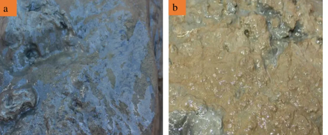
day because the excessive dissolved organic matter flows into the reservoir through two box culverts. 9 Fig. 3.1 Reservoir water (a) and bottom sediment (b) in the experiment, which were
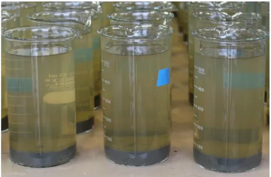
collected from an organically polluted reservoir. 12 Fig. 3.2 Approximately 70 tall beakers of 500 mL for water quality monitoring near the
bottom sediment were prepared for each case. 12 Fig. 3.3 The influent water into the organically polluted reservoir shown in Fig. 2.1
through the box culvert was used as the sample, including the high DOC con- centrations (a). The reductive sediment was used by directly providing the bot- tom mud sampled in the reservoir into tall-beakers (b), and the oxidative sedi- ments were prepared by exposing the sampled muds to aerated water in tall beakers for 2 weeks (c). 15 Fig. 3.4 Continuous measurements of DO and ORP for 20 days in case 1 and case 2. A
five-step process of decline in ORP is represented by points a, b, c, and d with each step having the following characteristics: Step 1: a linear decline from a to b; Step 2: a point of inflection at approximately 0 mV; Step 3: a steep decline from b to c; Step 4: a gradual decline from c to d; and Step 5: the state of equi- librium. The red broken line (case 1) and the black broken line (case 2) indicate results of linear regression formula for the drop from positive value to negative value in ORP. S is the slope of the linear line. R2 is the coefficient of determi- nation. 19 Fig. 3.5 Periodic measured results of NO3-N, NH4-N, PO4-P, sulfide, SO42-, TFe, and
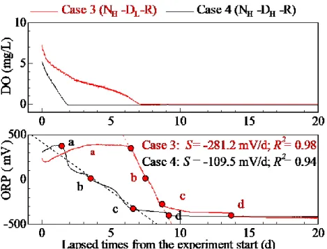
E254 during the experimental period in case 1 and case 2. Error bar standards are one standard error from the mean. The red solid line (case 1) and the black solid line (case 2) indicate results of the regression formula using logarithmic function for temporal changes in the concentrations of NH4-N and PO4-P. The regression coefficients of logarithmic trend lines of NH4-N and PO4-P were shown in parentheses. R2 is the coefficient of determination. 20 Fig. 3.6 Continuous measurements of DO and ORP for 20 days in case 3 and case 4. A
five-step process of decline in ORP is represented by points a, b, c, and d with each step having the following characteristics: Step 1: a linear decline from a to b; Step 2: a point of inflection at approximately 0 mV; Step 3: a steep decline from b to c; Step 4: a gradual decline from c to d; and Step 5: the state of equi- librium. The red broken line (case 3) and the black broken line (case 4) indicate results of linear regression formula for the drop from positive value to negative
iv
value in ORP. S is the slope of the linear line. R2 is the coefficient of determi- nation. 23 Fig. 3.7 Periodic measured results of NO3-N, NH4-N, PO4-P, sulfide, SO42-, TFe, and
E254 during the experimental period in case 3 and case 4. Error bar standards are one standard error from the mean. The red solid line (case 3) and the black solid line (case 4) indicate results of linear regression formula for temporal changes (increase or decrease) in concentrations of NO3-N, NH4-N and PO4-P, and the values in parentheses denote the gradients of approximate straight lines.
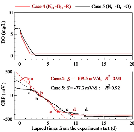
S is the slope of the linear line. R2 is the square of the correlation coefficient. 24 Fig. 3.8 Continuous measurements of DO and ORP for 20 days in case 4 and case 5. A
five-step process of decline in ORP is represented by points a, b, c, and d with each step having the following characteristics: Step 1: a linear decline from a to b; Step 2: a point of inflection at approximately 0 mV; Step 3: a steep decline from b to c; Step 4: a gradual decline from c to d; and Step 5: state of equilib- rium. The red broken line (case 4) and the black broken line (case 5) indicate results of linear regression formula for the drop from positive value to negative value in ORP. S is the slope of the linear line. R2 is the coefficient of determi- nation. 27 Fig. 3.9 Periodic measured results of NO3-N, NH4-N, PO4-P, sulfide, SO42-, TFe, and
E254 during the experimental period in case 4 and case 5. Error bar standards are one standard error from the mean. The red solid line (case 4) and the black solid line (case 5) indicate the approximately straight line for temporal change of concentrations, except for PO4-P in case 5, which can be approximated by the logarithmic trend line. The values in parentheses denote the regression co- efficients of logarithmic trend line for PO4-P in case 5. S is the slope of the linear line. R2 is the square of the correlation coefficient. 30 Fig. 3.10 Continuous measurements of DO and ORP for 25 days in case 5 and case 6. A
five-step process of decline in ORP is represented by points a, b, c, and d with each step having the following characteristics: Step 1: a linear decline from a to b; Step 2: a point of inflection at approximately 0 mV; Step 3: a steep de- cline from b to c; Step 4: a gradual decline from c to d; and Step 5: the state of equilibrium. The red broken line (case 5) and the black broken line (case 6) indicate results of linear regression formula for the drop from positive value to negative value in ORP. S is the slope of the linear line. R2 is the coefficient of determination. 33 Fig. 3.11 Periodic measured results of NO3-N, NH4-N, PO4-P, sulfide, SO42-, iron ion,
and E254 during the experimental period in case 5 and case 6. Error bar stand- ards are one standard error from the mean. The red solid line (case 5) and the black solid line (case 6) indicate the approximately straight line for NH4-N and the logarithmic trend line for PO4-P. The regression coefficients of loga- rithmic trend lines of PO4-P were shown in parentheses. S is the slope of the linear line. R2 is the coefficient of determination. 34 Fig. 4.1 Seasonal change in daily rainfall and transparency in 2015 and 2016. 41 Fig. 4.2 Seasonal data for water quality in 2015. 42
v
Fig. 4.3 Seasonal data for water quality in 2016. 43 Fig. 4.4 Bottom sedimentary surface samples were collected from the target water body
earlier than stratification time. The different colors of bottom mud is considered as a sign of the redox state of sediment, (a) in which brown color indicates that sedimentary surface is in oxidative state, (b) while gray color shows that it is in reductive state. 47 Fig. 4.5 Field observations of DO, ORP, NO3-N, NH4-N, PO4-P, sulfide,SO42-, E254,
and TFe at the bottom in 2015. S is the slope of linear line. R2 is the coefficient of determination. Dates in rectangle frames denote the data period used for cal- culating regression lines. 49 Fig. 4.6 Field observations of DO, ORP, NO3-N, NH4-N, PO4-P, sulfide,SO42-, E254,
and TFe at the bottom in 2016. S is the slope of linear line. R2 is the coefficient of determination. Dates in rectangle frames denote the data period used for cal- culating regression lines. 50 Fig. 4.7 Schematic of the ecosystem model. 57 Fig. 4.8 The relationship between light extinction coefficient and transparency for 2015
and 2016. 63 Fig. 4.9 Comparison of the measured chl.a, NO3-N, and NH4-N values with calculated
values using the general model (green lines) and the improved model (blue lines) in 2015 at the water surface. 67 Fig. 4.10 Comparison of the measured chl.a, NO3-N, and NH4-N values with calculated
values using the general model (green lines) and the improved model (blue lines) in 2016 at the water surface. 68 Fig. 4.11 Comparison of the measured values of DO, NO3-N, NH4-N, PO4-P, and sulfide
with calculated values using the general model (green lines) and the improved model (blue lines) in 2015 at the depth of 7 m. 72 Fig. 4.12 Comparison of the measured values of DO, NO3-N, NH4-N, PO4-P, and sulfide
with calculated values using the general model (green lines) and the improved model (blue lines) in 2016 at the depth of 7 m. 73 Fig. 4.13 Comparison of the measured values of DO, NO3-N, NH4-N, PO4-P, and sulfide
with calculated values using the general model (green lines) and the improved model (blue lines) in 2015 at the depth of 8 m. 74 Fig. 4.14 Comparison of the measured values of DO, NO3-N, NH4-N, PO4-P, and sulfide
with calculated values using the general model (green lines) and the improved model (blue lines) in 2016 at the depth of 8 m. 75 Fig. 4.15 Comparison of the measured values of water temperature (WT) with calculated
values using the improved model (blue lines) in 2015 at the depths of 0 m, 1 m, 2 m, 3 m, 4 m, 5 m, and 6 m. 79
vi
Fig. 4.16 Comparison of the measured values of water temperature (WT) with calculated values using the improved model (blue lines) in 2016 at the depths of 0 m, 1 m, 2 m, 3 m, 4 m, 5 m, and 6 m. 80 Fig. 4.17 Comparison of the measured values of DO with calculated values using the
general model (green lines) and the improved model (blue lines) in 2015 at the depths of 0 m, 1 m, 2 m, 3 m, 4 m, 5 m, and 6 m. 81 Fig. 4.18 Comparison of the measured values of DO with calculated values using the
general model (green lines) and the improved model (blue lines) in 2016 at the depths of 0 m, 1 m, 2 m, 3 m, 4 m, 5 m, and 6 m. 82 Fig. 4.19 Comparison of the measured values of NO3-N with calculated values using the
general model (green lines) and the improved model (blue lines) in 2015 at the depths of 0 m, 1 m, 2 m, 3 m, 4 m, 5 m, and 6 m. 83 Fig. 4.20 Comparison of the measured values of NO3-N with calculated values using the
general model (green lines) and the improved model (blue lines) in 2016 at the depths of 0 m, 1 m, 2 m, 3 m, 4 m, 5 m, and 6 m. 84 Fig. 4.21 Comparison of the measured values of NH4-N with calculated values using the
general model (green lines) and the improved model (blue lines) in 2015 at the depths of 0 m, 1 m, 2 m, 3 m, 4 m, 5 m, and 6 m. 85 Fig. 4.22 Comparison of the measured values of NH4-N with calculated values using the
general model (green lines) and the improved model (blue lines) in 2016 at the depths of 0 m, 1 m, 2 m, 3 m, 4 m, 5 m, 6 m. 86 Fig. 4.23 Comparison of the measured values of PO4-P with calculated values using the
general model (green lines) and the improved model (blue lines) in 2015 at the depths of 0 m, 1 m, 2 m, 3 m, 4 m, 5 m, 6 m. 87 Fig. 4.24 Comparison of the measured values of PO4-P with calculated values using the
general model (green lines) and the improved model (blue lines) in 2016 at the depths of 0 m, 1 m, 2 m, 3 m, 4 m, 5 m, and 6 m. 88 Fig. 4.25 Comparison of the measured values of sulfide with calculated values using the
improved model (blue lines) in 2015 at the depths of 0 m, 1 m, 2 m, 3 m, 4 m, 5 m, and 6 m. 89 Fig. 4.26 Comparison of the measured values of sulfide with calculated values using the
improved model (blue lines) in 2016 at the depths of 0 m, 1 m, 2 m, 3 m, 4 m, 5 m, and 6 m. 90
vii
LIST OF TABLE CAPTIONS
Table 3.1 Initial experimental conditions. 15 Table 3.2 Summary of laboratory experimental results of a five step process of decline
in ORP representing by ORP values (mV)and biochemical reactions corre- sponding to these steps. 36 Table 4.1 Correlation matrix of NH4-N, PO4-P, TFe, E254, SO42-
, and sulfide at the depth of 8 m in 2015. 53 Table 4.2 Correlation matrix of NH4-N, PO4-P, TFe, E254, SO42-
, and sulfide at the depth of 8 m in 2016. 53 Table 4.3 Set values of parameters concerned with the first-order rate constants of bi-
ochemical reactions. 65 Table 4.4Setting values of the mass ratios of nitrogen, phosphorus, TOD to carbon. 66 Table 4.5. Nash-Sutcliffe coefficients (NS) and root mean squared error (RMSE) be-
tween observed values and calculated values using the improved model and the general model in terms of Chl.a, NO3-N, and NH4-N at water surface in 2015 and 2016. 69 Table 4.6 Nash-Sutcliffe coefficients (NS) and root mean squared error (RMSE) be-
tween observed values and calculated values using the improved model and the general model in terms of DO, NO3-N, NH4-N, PO4-P, and sulfide at depths of 7 m and 8 m in 2015. 76 Table 4.7 Nash-Sutcliffe coefficients (NS) and root mean squared error (RMSE) be-
tween observed values and calculated values using the improved model and the general model in terms of DO, NO3-N, NH4-N, PO4-P, and sulfide at depth of 7 m and 8 m in 2016. 76
- 1 -
Chapter 1 Introduction
In low-lying agricultural areas in Japan, human activities and agriculture have relied heavily on closed water bodies such as marshes, lakes, creeks, and reservoirs as primary water resources. However, these water bodies are increasingly threatened by the excessive inflow of domestic, agricultural, or livestock wastewater containing high levels of organic matter, dis- solved inorganic nitrogen (DIN), and dissolved inorganic phosphorus (DIP) (Ramírez-Zierold et al., 2010; Aloe et al., 2014; Withers et al., 2014). These inflow loadings damage water re- sources through organic pollution and eutrophication. In organically polluted closed water bod- ies, the water column can be divided into two layers as shown in Fig. 1.1, hypolimnion and epilimnion, by the formation of thermal stratification during summer (Elçi, 2008; Hasan et al., 2013). Each layer can be characterized by different water quality dynamics derived from bio- chemical reactions and hydraulic phenomena. In the hypolimnion, dissolved oxygen (DO) can- not be produced by photosynthesis of phytoplankton because of insufficient underwater light intensity and the thermocline restraints the vertical transport of DO from the surface layer down
Fig. 1.1 Structure of water column due to formation of thermal stratification.
EPILIMNION
HYPOLIMNION
8 7 6 5 4 3 2 1 0
0 10 20 30 40
Water temperature ( oC)
Water depth (m)
- 2 -
to the bottom, resulting in the occurrence of anoxic water, which is one of the most serious aquatic environmental problems (Sahoo and Luketina, 2006). This state causes the death of aquatic biota by oxygen deprivation and acceleration of eutrophication by nutrients release from the bottom sediment, such as nitrogen and phosphorous (Nürnberg, 1994; Prairie et al., 2001;
Nowlin et al., 2005). In addition, the generation of hydrogen sulfide and the accumulation of sludge, including metal sulfide and undecomposed organic matter on the bottom, cause damage to the aquatic environment (Bagarinao, 1992). These aquatic environmental phenomena strongly correlate with the biochemical reactions under anaerobic conditions, such as iron re- duction causing the leaching of phosphorus or sulfate reduction causing the production of hy- drogen sulfide (Almeida et al., 2006 ; Lee et al., 1977; Parker and Beck, 2003; Martins et al., 2014). In the epilimnion, nutrients as well as optimal underwater light intensity increase phy- toplankton concentrations, resulting in the excessive growth of blue-green algae (Cloern, 1999;
Boesch, 2002), known as algal blooms, in summer. Consequently, the overgrowth of algae causes environmental problems such as landscape damage, obstructions to agricultural water use, and generation of fetid water (Jahan et al., 2010). The increase of phytoplankton in the epilimnion becomes the primary factor in the formation of hypolimnion by reducing transpar- ency. Nutrients eluted from the bottom sediment under anaerobic conditions can lead to further eutrophication. Therefore, the analysis of phytoplankton, nitrogen, phosphorus, and DO in the hypolimnion and epilimnion is essential for formulating environmental preservation measures and for preventing algae overgrowth and anoxia. This analysis involves not only field observa- tions for temporal or spatial change of water quality, but also aquatic environmental evaluation using hydraulic and water quality models.
The aquatic environmental analysis for the conservation and restoration of water bodies through not only risk analysis of environmental changes, but also impact assessment of water quality improvement measures is an effective approach to apply water quality prediction mod- els that rely on both hydraulic transport of mass and biochemical changes in water quality. In general, the former follows the advection-diffusion equation of material and the latter is con- sidered an ecosystem model formulating the material circulation of carbon, nitrogen, and phos- phorus based on the biochemical reactions within the aquatic system. Ecosystem models have
- 3 -
been widely applied for water quality assessment as essential tools to determine the seasonal changes in DO and phytoplankton levels in eutrophic water bodies (Prokopkin et al., 2010;
Özkundakci et al., 2011). However, in lakes and reservoirs that exhibit long-term anoxification, the predicted results of nutrient salts are quite different from the observed values (Smith et al.
2014) because the internal loading of nitrogen and phosphorus under anaerobic conditions are not expressed well in a general ecosystem model. In addition, there has been no study that incorporated sulfide as a state variable of the ecosystem models because its dynamic character- istics have not been quantitatively estimated through on-site water quality surveys. To address these issues, the ecosystem model needs to reflect the dynamic characteristics of water quality in anaerobic respiration processes, including denitrification, iron reduction, and sulfate reduc- tion. However, there have been a few studies that quantitatively estimated the water quality dynamics in the hypolimnion of actual water bodies from a biochemical perspective. Limited research has been done for increasing the levels of phosphate-phosphorus (PO4-P), ammonium- nitrogen (NH4-N), and sulfide near the bottom bed in a greatly reductive state caused by the long-term depletion of oxygen.
In aquatic environments, reduction half-reactions through inorganic compounds con- taining oxygen under anaerobic conditions occur in stages, and begin with high oxidation reduction potential (ORP) (Gordon and Higgins, 2007). The major biochemical reductions (beginning with the most important) are: denitrification, iron reduction, sulfate reduction, and methane fermentation. From the thermodynamic point of view, it is possible to determine at which stage a reduction half-reaction occurs by measuring the ORP and pH, and it is also pos- sible to quantitatively evaluate a reduction reaction that occurs under anaerobic conditions.
However, in actual water bodies, many oxidation-reduction reactions overlap through a variety of microorganisms, and they create complex reaction systems that are difficult to understand.
For example, Li et al. (2016) showed that ORP was effective as an index to quantitatively rep- resent phosphorus release from the bottom sediment, but there are many aspects that should be studied in order to actually perform such quantitative evaluations using ORP. Moreover, alt- hough estimating ORP in water bodies under oxygen deficient conditions is widely studied, very little research has been done on the hypoxic state of the hypolimnion in actual water bodies.
- 4 -
In light of such a background, Harada et al. (2014) performed water quality monitoring in an organically polluted reservoir with the observation point located 1 m directly above the bottom. The results showed that it was possible to model the dynamic state of ORP under an- aerobic conditions with a logistic curve, and to evaluate the change with time in sulfide, NH4- N, and PO4-P in relation to ORP with a linear regression model. However, there has been no study of water quality dynamics near the bottom bed in a greatly reduced state caused by long- term depletion of oxygen, and which is strongly impacted by the bottom material. Nishioka et al. (2016) monitored the water quality near the bottom material under anaerobic conditions by forming an anoxic water state inside a cylindrical tank with a 30 cm diameter and 100 cm height.
The aim of their research was to clarify the biochemical characteristics of water quality dynam- ics, including a consideration of the impact of the bottom material through an experimental approach. As a result, they modeled the dynamics of ORP in an anoxic state using a logistic curve, as they simultaneously quantitatively evaluated the increase in PO4-P, NH4-N, and sul- fide, based on a non-linear regression model. In addition, the results also revealed that the re- gression coefficients of these models can be dependent on the initial concentration of NO3-N or the organic matter in the water sample used in the experiment. However, this dependency has not been quantitatively evaluated.
It is known that denitrification, which occurs initially by anaerobic decomposition of organic matter, greatly impacts the reduction half-reaction that takes place in later stages. Based on this feature, Oniki et al. (2017) performed beaker-scale water quality monitoring to study the dynamic properties of NH4-N, PO4-P, and sulfide by investigating NO3-N in the initial an- aerobic stage after oxygen was depleted. The results revealed that the dynamics of ORP in the anoxic state are characterized by a five step process of decline, and that the initial NO3-N could be a water quality factor regulating the speed of this decline. They also explained the process of increase in PO4-P, NH4-N, sulfide, and dissolved organic carbon (DOC) under anaerobic conditions in relation to the change with time in NO3-N and the staged decline in ORP. Besides, they evaluated the characteristics of these changes based on linear regression and non-linear regression models and described the impact of the initial NO3-N on the characteristics of the water quality dynamics under anaerobic conditions.
- 5 -
To quantitatively estimate the anaerobic respiration processes, besides the impact of the initial NO3-N, this study focused on the concentration of dissolved organic matter (DOM) and the redox state of the bottom sediment as the factors affecting water quality dynamics under the anoxic condition. The biochemical reactions, such as denitrification, iron reduction, sulfate re- duction and methane fermentation, occur as reductive half-reactions carried out by anaerobic microorganisms, while oxidative half-reactions occur as well with organic matter as the electron donor (Krevš and Kučinskienė, 2009; Polubesova and Chefetz, 2014). DOM is thus the easiest form of organic matter for anaerobic microorganisms to use as a respiratory substance, and this has a major effect on the variability in water quality associated with the development of anoxia.
The inflow load of humic acids from forested areas and agricultural regions has been identified as one cause of the organic pollution in water bodies. Therefore, a quantitative investigation of the effect of a high DOM concentration caused by the anaerobic decomposition of organic mat- ter on water quality dynamics in water bodies would be highly significant. In closed water bod- ies in warm regions, anoxia develops because of thermal stratification formation during the warm periods in spring and summer, which dissipates with the vertical mixing due to water surface cooling during fall and winter. The sediment surface changes from reductive to oxida- tive (Fig. 1.2) because of the aerobic conditions near the bottom in fall and winter, and this oxidative state is maintained until hypoxic water masses form in spring. The sediment surface comprises an oxidative layer during the early stage of thermal stratification; thus, it is important to conduct the quantitative evaluation through studying the effect of redox state of sediments
Fig. 1.2 Sediment surface changes from reductive (a) to oxidative (b) in fall and winter due to the vertical mixing leading to aerobic conditions near the bottom.
a b
- 6 - on the activity of anaerobic microorganisms.
This study focuses on the environmental analysis in a closed water body where the epi- limnion and hypolimnion could be formed due to thermal stratification. The major aims are not only to quantitatively estimate water quality dynamics derived from anaerobic respiration based on laboratory experiments and field observations, but alsoto improve the water quality predic- tion model by taking account of both the generation of sulfide and the elution of PO4-P and NH4-N from the bottom sediment. This study has two important parts as following.
First, the water quality dynamics under anaerobic conditions were examined through beaker-scale water quality monitoring in order to understand aquatic environmental deteriora- tion due to the anoxic state in an organically polluted water body. The outcome of this labora- tory experiment, which was focused on the dynamic properties of NO3-N, NH4-N, PO4-P and sulfide above the sediment from the anaerobic respiration activity point of view, was described in Chapter 3. The specific aims of this chapter were to quantitatively estimate the impacts of the oxidative/reductive state of the sediment surface and the high/low concentrations of dis- solved organic matter on the dynamic properties of water quality under anaerobic conditions.
The beaker-scale water quality monitoring was carried out through continuous measurements of DO and ORP, as well as periodic observations of water quality parameters for six cases that were composed from combinations of three experimental conditions: concentration of DOC, redox state of the sediment, and concentration of NO3-N. Characteristics of the temporal change in ORP under anoxic conditions were quantitatively estimated by relating anaerobic respiration processes, including denitrification, iron reduction, and sulfate reduction. Also, by comparing these six experimental conditions, it was examined that the influence of high DOC concentra- tions in water and oxidative states of the bottom mud accelerated on the increases of NH4-N, PO4-P and sulfide due to anaerobic state.
Next, this study focuses on the water quality dynamics in an organically polluted reser- voir exhibiting long-term anoxification using two approaches: (1) field observations of seasonal changes in vertical profiles of DO, nitrogen, phosphorus, and sulfide, and (2) construction of a water quality prediction model based on an ecosystem model incorporated with anaerobic bio- chemical processes. The outcome of these research approaches was described in Chapter 4. In
- 7 -
this chapter, this research particularly considered that the redox state of the bottom sediment surface, when anoxification began to occur, greatly affected the water quality dynamics caused by gradual reductive reactions under anaerobic conditions. To achieve this aim, characteristics of the water quality dynamics were examined based on the observed data for two years. Also, this study proposed the modifications of the conventional ecosystem model based on the finding obtained by the field observations in order to highly improve the calculation accuracy of NH4- N, PO4-P and sulfide. By simulating the observed data, this study indicated that the upgraded water quality prediction could be used to quantitatively estimate the water environment dynam- ics in organically polluted water bodies.
Finally, general conclusions and recommendations for general implementation of above described research activities involving the laboratory experiment, water quality survey, and constriction of simulation model were pointed out in Chapter 5.
- 8 -
Chapter 2 Study area
The target water body is a regulating reservoir on the Ito Campus of Kyushu University, Japan, with water surface area of ca. 19,300 m2, pondage of ca. 63,000 m3, and maximum water depth of ca. 8 m (Fig. 2.1). This reservoir, located in the deforestation area, was created for rainfall storage. In summer, the water level is maintained at a high level because the reservoir functions as a source of irrigation water to the downstream paddy fields. During rainfall, a large amount of water flows into the reservoir through two box culverts from the catchment area and the stored water is discharged simultaneously from the spillway (Fig. 2.2). The logged wood chips yielded at the time when the deforestation have occurred into the campus, are covered with the developed land including the neighborhood of the targeted reservoir. As a result, ex- cessive levels of dissolved organic matter from the humified wood chips flow into the pond through two box culverts during rainfall and high inflow of humic acid causes a dark reddish- brown color in the water (Fig. 2.2). In addition, earth and sand used in the campus construction flow into the reservoir through box culverts during heavy rainfall resulting in turbid water. The insufficient underwater light intensity caused by dissolved and particulate matter leads to ther- mal stratification from summer to autumn, resulting in the formation of the hypolimnion with the decline of DO levels. Anoxic water could occur in depths > 2 m by strong thermal stratifi- cation in summer and the anoxification above the bottom bed could be maintained over six months (Harada et al., 2014; Nguyen et al., 2015). The thermal stratification would also cause seasonal increases in ammonium, phosphate, and sulfide levels in the hypolimnion and deposi- tion of mud at the bottom (Nguyen et al., 2015).
- 9 -
Fig. 2.1 The target reservoir and its two box culverts, Ito campus of Kyushu Univer- sity, Japan.
.
Fig. 2.2 The water color in the target reservoir changes to brown color in a heavy rain day because the excessive dissolved organic matter flows into the res- ervoir through two box culverts. The stored water is discharged concur- rently from the spillway.
The target reservoir Box culvert 2
Box culvert 1
100m
0 200m 300m 400m
N
W E
S
The target reservoir in a rainy day
Spillway Box culvert 2
- 10 -
Chapter 3 Experimental study on the influence of DOM and bottom sediment redox state on water quality dynamics under anaerobic conditions
3.1 Introduction
In this chapter, laboratory experiments were conducted to evaluate the influence of the concentration of DOM and the redox state of the sediment as factors affecting water quality dynamics in anoxic water bodies. The same experimental method used by Oniki et al. (2017), namely beaker-scale water quality monitoring, was used in this study to obtain basic knowledge of the biochemical characteristics related to the water quality dynamics in the process of water interaction with the bottom material. This interaction took place through the activities of mi- croorganisms. Further, this study was conducted in terms of a high DOC concentration and redox state of the sediment surface. The closed water body assumed in this study was a rela- tively deeper lake or reservoir where the two layers of the epilimnion and hypolimnion could be formed due to thermal stratification. Moreover, this study focused on the water depth range close to the bottom bed in the hypolimnion, where the static state could be maintained by being entirely isolated from surface wind-mixing. In such a range, water quality dynamics are unaf- fected by hydrodynamic mass transport and depend only on the biochemical matter cycle.
Therefore, it is considered that the water quality dynamics, which are similar to actual phenom- ena in the hypolimnion, can be generated in beaker-scale experiment.
3.2 Experimental methods and conditions
The environmental water and bed material used in the beaker-scale water quality mon- itoring were sampled from the target study area, a regulating reservoir. This reservoir had turned yellowish brown owing to the inflow of humic acid, and the hypolimnion with anoxic water was formed in the depth range of deeper than about 2 m by the strong thermal stratification in the summer. This study consisted of a laboratory experiment performed by filling a beaker with stored water and bottom sediment from an actual organically polluted reservoir, keeping this filled beaker in a dark place insulated from the atmosphere so that its contents are in anoxic
- 11 -
condition, and then measuring the change in the water quality with time under anaerobic con- ditions. This experiment was adopted because it simply enables the water quality monitoring directly above the bottom material. In addition, the beaker-scale experiments enable choosing and focusing on the specific condition of various environmental factors affecting water quality dynamics, and then provides the basic information to quantitatively clarify their characteristics under the anaerobic state. In this study, water quality was monitored in multiple cases with the initial DOC concentrations and the initial oxidation-reduction state of the surface layer of the bottom material as the experimental conditions. This was done in order to study the impact that these two environmental factors have on water quality dynamics under anaerobic conditions. A statistical analysis was performed using linear and non-linear regression models of the PO4-P, NH4-N, and sulfide time series data, and the change in the characteristics of the entire water environment with time was considered by focusing on the experiment start timing and the rates of increase in the concentrations of these compounds. Furthermore, the calculations were con- ducted based on the relationship of these parameters with other water quality parameters, such as ORP, NO3-N, and the quantity of the existed organic matter.
3.2.1 Preparation of laboratory experiments under anaerobic conditions
The laboratory experiments were performed using actual reservoir water and bed ma- terial (Fig. 3.1), in which organic pollution had been detected due to an inflow loading of humic acid, and during the summer when oxygen depletion was accompanied by thermal stratification.
A tall, 500 mL beaker filled with bed material (approximately 100 mL) and water (approxi- mately 400 mL), sampled from the same reservoir, were left standing in a dark room at a con- stant temperature of 20oC(Fig. 3.2) to inhibit oxygen production by photosynthesis. In addition, the water surface in each beaker was covered with liquid paraffin to block the supply of oxygen from the atmosphere in order to prepare the sample water in an anoxic state. As described in detail in the next section, water quality monitoring was conducted under the 6 cases of experi- mental conditions, and approximately 70 beakers were prepared for each case. For each case, the changes in DO and ORP over time were continuously monitored in one randomly selected beaker from the available 70 tall-beakers. In addition, the other water quality parameters related to the organic
- 12 -
Fig. 3.1 Reservoir water (a) and bottom sediment (b) in the experiment, which were collected from an organically polluted reservoir.
Fig. 3.2 Approximately 70 tall beakers of 500 mL for water quality monitoring near the bottom sediment were prepared for each case.
a b
- 13 -
pollution (as described below) were measured periodically using the other remaining tall beakers.
When preparing the samples, water was poured carefully to avoid agitating the bottom layer and making the samples murky. Samples were also left to sit for approximately 12 hours prior to starting the experiment to ensure that even the small floating particles would have no effect on the results of the water quality monitoring. According to the water quality monitoring results (Harada et al., 2014) for the reservoir where the sampling was conducted, anoxia at the bottom level has been continuously observed over the course of 6 to 7 months. If laboratory testing is used for such long periods, the amount of water samples required for the scheduled measurement of water quality would be enormous, even if it was only on a weekly basis. The same observations showed that when one month had passed after anoxia, there was a strong reduction in ORP by approximately 400 mV, and a striking increase in the concentrations of nutritional salts and sulfides in the water, that was confirmed over a 1 to 2 month period. In light of these findings, the implementation period of the laboratory experiment was estimated to be approximately 2 months in order to focus on the changes over time in water quality char- acteristics resulting from the shift in aerobic to anaerobic conditions.
3.2.2 Outlines of water quality monitoring
Fluorescent DO and ORP meters were used for the continuous measurements, and in addition, both DO and ORP data were logged at 20-minute intervals. The fluorescent DO elec- trode has a fast response time and superb measurement accuracy and repeatability, enabling a continuous and stable measurement in such a still fluid environment. Also, the ORP measure- ment electrode was made of platinum, and the reference electrode was made of silver chloride, while potential (Eh) conversions using a hydrogen standard electrode was not performed. How- ever, an approximate Eh value was calculated by adding 200 mV to the measured value.
Measurements were taken every 3 days during the first month of the experiment, and every 7 days during the second month of the experiment. As a result, measurement data was acquired between 14 to 17 times during the two-month period of the experiment. The water quality was analyzed three to five times with respect to the scattering between samples. For
- 14 -
water quality analysis, samples with liquid paraffin were removed using lipophilic and hydro- phobic oil absorption sheets. The major water quality parameters in this study were NO3-N, NH4-N, PO4-P, SO42, sulfide, total iron ion (TFe) (sum of Fe2+ and Fe3+), total organic carbon (TOC), DOC, and ultraviolet light absorption at 254 nm of wavelength (E254). These parame- ters were measured as follows: (a) both NO3-N and SO42 were measured by an ion chromato- graph (DX-320, Dionex); (b) PO4-P and total iron ion were analyzed by absorption spectropho- tometry based on the ascorbic acid reduction-molybdenum blue method, and the 2,4,6-tris (2- pyridyl)-1,3,5-triazine method, respectively, using the (DR5000, HACH) spectrophotometer;
(c) sulfide was measured as S2 ion concentration by the DR500 based on the ethylene blue method, and this analysis included ions liberated from hydrogen sulfide, hydrogen sulfide ions, and soluble metal sulfides (including iron sulfide), due to the presence of sulfuric acid; (d) NH4- N was determined by using coulometric titration-type ammoniacal nitrogen meter (AT-2000, Central Kagaku Corp); (e) TOC and DOC were measured by a TOC analyzer (Sievers 900, GE Analytical Instruments) based on a wet ultraviolet oxidation reaction and selective membrane conductometric technology; and (f) E254 was measured by a (DR5000, HACH) spectropho- tometer. E254 was used as an indicator of humic acids and other dissolved organic matter to act as an additional water quality parameter.
3.2.3 Experimental conditions
The above laboratory experiments (monitored by both continuous and periodic meas- urements) were carried out for six cases with different initial conditions of three parameters;
NO3-N concentration, DOC concentration, and oxidation-reduction state of the bottom material surface. The details of the experimental conditions of cases 1 to 6 are summarized in Table 2.1.
The continuous water quality monitoring and the scheduled water quality measurement were started 12 hours after the preparation of the samples to remove the influence of tiny soil particles on the water quality measurements. These particles are generated when water is injected into the beakers causing the bottom sediment to spread all over the beaker. Cases 1 and 2 were set in order to examine the impacts of low and high DOC concentrations on the biochemical dy- namics of water quality parameters, such as NH4-N, PO4-P and sulfide, under both low NO3-N
- 15 -
Table 3.1 Initial experimental conditions
Case study NO3-N
(mg/L)
DOC (mg/L)
Redox state of sediment ORP(mV) Case 1 NL-DL-R 0.098 Low 4.407 Low 132 Reduction Case 2 NL-DH-R 0.087 Low 16.560 High 121 Reduction Case 3 NH-DL-R 0.337 High 3.958 Low 139 Reduction Case 4 NH-DH-R 0.319 High 16.980 High 153 Reduction Case 5 NH-DH-O 0.326 High 14.733 High 29 Oxidation Case 6 NH-DL-O 0.530 High 4.733 Low 94 Oxidation
Fig. 3.3 The influent water into the organically polluted reservoir shown in Fig. 2.1 through the box culvert was used as the sample, including the high DOC concentrations (a). The reductive sediment was used by directly providing the bottom mud sampled in the reservoir into tall-beakers (b), and the oxi- dative sediments were prepared by exposing the sampled muds to aerated water in tall beakers for 2 weeks (c).
- 16 -
concentration and reduction state. Also, cases 3 and 4 were set in order to compare the influence of low and high DOC concentrations under both high NO3-N concentration and reduction state conditions. Moreover, the impacts of oxidation state on water quality dynamics were examined through cases 5 and 6 with high and low DOC, respectively, and with high NO3-N concentration in both cases.
Samples of cases 2, 4 and 5, in which the initial DOC concentrations were high, were prepared in the range of 14 to 17 mg/L by sampling the water in the box culvert flowing into the reservoir after a heavy rainy day (Fig. 3.3a). This inflow of water turned dark reddish-brown from the humic acid. On the other hand, the low DOC concentrations in cases 1, 3, and 6 were set around 4 mg/L using the reservoir’s water. In addition, the bottom materials in cases 1 to 4 used sediments (Fig. 3.3b) that were in reductive states with negative ORP, as shown in Table 3.1.
The bottom material samples were obtained in the summer when the anoxic state above the bottom bed had been maintained beyond 5 months. The oxidative sediment in cases 5 and 6, as shown in Fig. 3.3c, which were initially positive (Table 3.1), were prepared by exposing the reductive bottom mud, which was sampled on the reservoir in summer, to aerated water in tall beakers for 2 weeks.
Furthermore, the initial NO3-N concentrations were adjusted using a nitrate ion standard solution. Here, the experimental results for the low DOC concentration conditions and the re- ductive bottom material by Oniki et al. (2017) were utilized as cases 1 and 3 in this study.
However, the experimental data in both cases (cases 1 and 3) did not include the results for total iron ion or E254. Thus, the causes of the phenomena resulting from the water quality dynamics under anaerobic conditions, especially nutrients and sulfide generation, were not fully clarified.
To understand clearly the changes in nutrients as well as sulfide under anaerobic conditions, E254 and total iron ion were added in periodic measurements of the other cases (cases 2, 4, 5, and 6).
3.3 Results and discussion
3.3.1 Lowering property of ORP under anoxic state
- 17 -
A comparison study was conducted in three stages to investigate the effects of experi- mental conditions, such as DOC concentration and the redox state of the sediment, and the effect of NO3-N on the water quality dynamics under anaerobic conditions (Oniki et al., 2017).
First, the variation in water quality due to different DOC concentrations was studied under the initial conditions of low NO3-N concentrations and reducing sediments. Next, the effect of DOC on water quality dynamics with high concentrations of NO3-N in the same reducing sediments was examined. Finally, the effects of high and low concentrations of DOC in oxidizing sedi- ments were studied.
This study then focused on the changes in the parameters over time by applying contin- uous monitoring of the DO/ORP, as shown in Figs. 3.4, 3.6, 3.8 and 3.10, and the periodic monitoring of the water quality parameters (NO3-N, NH4-N, PO4-P, sulfide, SO42, TFe, and E254), as shown in Figs. 3.5, 3.7, 3.9, and 3.11. As explained later, regardless of the experi- mental conditions, DO and ORP showed a marked drop 10–20 days after the experiment started, and then leveled off. Figs. 3.4, 3.6, 3.8 and 3.10 are graphic representations of the time lapse from the start of the experiment to 20 days later, which were created to clearly illustrate the changes in ORP during the anoxic period. The results of periodic water quality measurements illustrated in Figs. 3.5, 3.7, 3.9 and 3.11, 3in which the maximum and minimum values of anal- ysis of multiple samples were represented by error bars, and the water quality dynamics were represented by average sample values indicated by dots on the bar.
The results of the continuous measurement of DO and ORP under low DOC concentra- tions and reductive bottom material conditions (cases 1 and 3) were consistent with the results obtained by Oniki et al. (2017), which showed that after a hypoxic state of DO < 1.0 mg/L was attained, ORP decreased to approximately 400 mV in stages until it eventually reached equi- librium. According to their results, the dynamic properties of ORP after the decrease in DO can be summarized in 5 stages, as follows: Step 1 was the transition from an aerobic to an anaerobic state, and it was found that in this stage the decrease in ORP was delayed by the initial high concentration of NO3-N; Step 2 was the point of transition from an oxidative state to a reductive state caused by oxygen depletion, which conformed roughly to the point at which DO became zero; Step 3 was the stage of rapid decrease in ORP in a reductive state and, similar to Step 1,
- 18 -
the rate of decrease is inversely related to the initial NO3-N; Step 4 in which ORP decreased slowly, and this period of decrease was prolonged by high initial NO3-N concentrations; and Step 5 where ORP reached a state of equilibrium and leveled off at a constant rate with the lowest electric potential of about 400 mV, although the higher the initial NO3-N concentrations, the longer it took to reach equilibrium. The decline of ORP following the decrease of DO greatly impacts the phased transition of the reduction half-reactions accompanying organic matter de- composition by anaerobic microbes. Therefore, this study would examine the change with time in ORP while taking the dynamic properties of ORP as stated above into consideration.
3.3.2 Influence of DOC under low NO3-N and reductive bottom sediment
In this section, the influence of initial DOC concentration under low NO3-N and reduc- tive sediment conditions is discussed by comparing cases 1 and 2 based on the results illustrated in Figs. 3.4 and 3.5. First, similar to case 1, ORP in case 2 began to decline as soon as DO dropped to near zero. The rate of decline in ORP that was calculated up to Step 3 was 108.7 mV/d, according to the regression formula for case 1, and 89.2 mV/d for case 2. The values of the decline in the ORP slope are similar in cases 1 and 2, indicating that high or low concen- trations of DOC had no significant effect on the temporal change in ORP from Step 1 to Step 3. Step 4 showed a gradual drop in ORP during periods that differed depending on the DOC conditions (about 5 days in case 1 and about 2 days in case 2). The time required to reach Step 5, which is the point where the system reaches an equilibrium state, became shorter due to the high DOC concentration conditions. Among the main reductive reactions which occur in the actual water body, ORP produced by the sulfate reduction reaction should be about 350 mV (using ORP meter employing AgCl as the reference electrode), because it becomes limited by competition with other reductive reactions, such as denitrification (Whitmire and Hamilton, 2005). The results indicated that the point in time when ORP shifts to reach the equilibrium state (400 mV) at Step 5 matched the point in time when sulfide started to increase in both cases 1 and 2. It can also be confirmed that NO3-N decreased to zero at Step 4 and denitrification was completed before the ORP reached Step 5. Consequently, Step 5 is characterized as a pro- cess in which sulfide increases by sulfate reduction and is not limited by denitrification. In
- 19 -
Fig. 3.4 Continuous measurements of DO and ORP for 20 days in case 1 and case 2.
A five-step process of decline in ORP is represented by points a, b, c, and d with each step having the following characteristics: Step 1: a linear decline from a to b; Step 2: a point of inflection at approximately 0 mV; Step 3: a steep decline from b to c; Step 4: a gradual decline from c to d; and Step 5:
the state of equilibrium. The red broken line (case 1) and the black broken line (case 2) indicate results of linear regression formula for the drop from positive value to negative value in ORP. S is the slope of the linear line. R2 is is the coefficient of determination.
- 20 -
Fig. 3.5 Periodic measured results of NO3-N, NH4-N, PO4-P, sulfide, SO42-, TFe, and E254 during the experimental period in case 1 and case 2. Error bar stand- ards are one standard error from the mean. The red solid line (case 1) and the black solid line (case 2) indicate results of the regression formula using logarithmic function for temporal changes in the concentrations of NH4-N and PO4-P. The regression coefficients of logarithmic trend lines of NH4-N and PO4-P were shown in parentheses. R2 is the coefficient of determination.
0 0.2 0.4 0.6
0 1 2 3
0 0.2 0.4 0.6
0 200 400
0 5 10 15
0 4 8
0 10 20 30 40 50 60 70
0 0.4 0.8 1.2 NO3-N (mg/L)PO4-P (mg/L)NH4-N (mg/L)Sulfide (μg/L)SO42- (mg/L)TFe (mg/L)E254
Lapsed times from the experiment start (d) Case 1 ( NL -DL -R) Case 2 ( NL -DH -R)
Case 2 (0.533 mg/L); = 0.90 Case 1 (0.245 mg/L); = 0.86
Case 1 (0.033 mg/L); = 0.86 Case 2 (0.048 mg/L); = 0.54
R2 R2
R2 R2