ビッグバン元素合成とダークエネルギーの進化

(1)

九州大学学術情報リポジトリ

Kyushu University Institutional Repository

一政, 遼太郎

https://doi.org/10.15017/1806810

出版情報：Kyushu University, 2016, 博士（理学）, 課程博士バージョン：

権利関係：Fulltext available.

(2)

Thesis

Big Bang Nucleosynthesis and Evolution of Dark Energy

Theories of Particle Physics,

Nuclear Physics and Astrophysics/Astronomy, Department of Physics, Graduate School of Science,

Kyushu University

Advisor: Prof. Masa-aki Hashimoto March 2017

Ryotaro Ichimasa

(3)

Abstract

The standard model of cosmology based on the Big Bang theory is established as the theory which can reproduce many astrophysical phenomena because of dramatic improve- ments of observations in recent years. Cosmic Microwave Background (CMB) radiation, type Ia supernovae, abundances of light elements and determination of H₀ by observing the Cepheid variables are the representative observations. In particular, CMB is observed using WMAP satellite and Planck satellite up to the redshift,z ∼1000, which includes the oldest information we can currently obtain. These observations have revealed that only 4% of baryons is present as the component of the current universe. Others are consist of dark matter (28%) and dark energy (68%). In order to describe correctly the evolution of the universe, it is necessary to accurately predict the time evolution of these components.

Although current composition ratios among baryons, dark matter and dark energy are determined exactly, more detailed observation and analysis are required to clarify their properties.

Helium-4 and deuterium are the most important elements that are synthesized in the early universe: so-called Big Bang nucleosynthesis (BBN). Observation of helium-4 has large ambiguity because the primordial quantity is evaluated using models of chemical evolution of the galaxy. In addition, there exist crucial uncertainties for observations.

Two groups give diﬀerent observational results.

On the other hand, the abundance of deuterium is estimated from the absorption spectrum due to the backward quasar which is considered to be the primitive galaxy at the early stage of its formation; and the abundance is determined with very high accuracy.

In order to predict accurately these abundances of light elements which are assumed to be synthesized by BBN, it is necessary mainly to determine the nuclear reaction rates, the lifetime of neutrons, and the number of neutrinos.

Since the present universe is dominated by dark energy, the nature of dark energy characterizes the evolution of the universe. Clarifying its feature is one of the important studies in cosmology. There are many theoretical predictions as the candidates for dark energy. One of them is a cosmological term. It can be interpreted as a static dark energy which is introduced by Einstein. For the other candidates, dynamical dark energy models, such as quintessence field and phantom field, are also theoretically predicted. Thus, there

(4)

are many kinds of method to describe the characteristics of dark energy. In addition to these models, dark energy can also be characterized by using a modified gravity field theory and an equation of state. In recent years, many discussions are performed for the availability of gamma ray bursts to limit the properties of dark energy, in addition to adopt type Ia supernova data. The supernova data have been used to constrain the properties of dark energy. If gamma ray bursts become available, we can constrain the character with use of 7 times wider range of the redshift z <10.

It is assumed in these models that dark energy conserves its energy independently from other components. It is necessary to clarify the presence or absence of energy transport among them. There have been many studies on the interaction between dark energy and dark matter. Although, the latest observational data indicate that the interaction between them is not allowed, energy transport may exist between dark energy and photons may exist. Improvement of observational accuracy makes it possible to determine the temperature of the CMB photons at low redshift within 3% precision. Furthermore, it is suggested that the energy density of the CMB photons may not be conserved with 1σ confidence level. There have been proposed models with interaction between dark energy and photons which influence BBN. However, if there is an interaction between dark energy and photons, there arises a possibility of influencing Big Bang nucleosynthesis.

In the present study, firstly we investigate BBN. For the nuclear reaction rates of our calculations we adopt astrophysical nuclear reaction rates (NACRE-II) using the latest experimental value and 880.1 ± 1.1 s (J. Beringer et al. 2013) for neutron lifetime. We take observations of Izotovet al. (2013) and Aver et al. (2013) for helium-4 abundance.

Our result is consistent with the observational value of Aver et al. (2013). As for the observational value of Izotov et al., if we include degenerate electron neutrinos we can find a plausible range of the baryon density with 1σ confidence level.

Secondly, using a specific equation of state, we investigate the density evolution of dark energy to clarify its feature in the low redshift universe. Taking account of the observational values of type Ia supernovae and gamma ray bursts, we can exclude a dark energy model in which cosmological behavior changes from a phantom-like model to quintessence-model with 2.4σ confidence level.

(5)

1 Introduction

What is the composition of our universe? How did the universe begin and evolve? These are the most basic questions. In the past few decades, our common sense for the universe has changed drastically. Einstein established the theory of general relativity and enabled a physical approach to the universe in 1916. The theory described not only the gravitational field, but also the evolution of the universe. Moreover, the theory predicts the steady, expanding, and contracting universe. Thereafter, George Gamow introduced the Big Bang model which describes the universe from the beginning to the end. Big Bang model has predicted three observational evidences:

1) Our universe is not stationary, but expanding.

2) Light elements were synthesized at the early universe.

3) Cosmic Microwave Background Radiation is a relic of hot Big Bang.

Currently, there are many observational results that roughly support above predictions.

However, these arise some cosmological problems, such as lithium problem, cosmological constant problem, flatness problem, horizon problem, and monopole problem. It is well known that the last three problems can be solved by adopting an inflation model. However, the others remain as unsolved serious issues. To make matters worse, recent observational results on the abundance of light elements cause a new serious problem.

In Sec. 1 we introduce the conventional approach to the cosmology and current problems what we focus on. In Sec. 2 we summarize the current situation of the Big Bang nucleosynthesis and observed abundances of light elements. In Sec. 3 we present our models and calculational results for dark energy, which is the alternative conjecture of a cosmological constant. Summary and discussions are given in Sec. 4.

1.1 Historical Review

Newton’s gravitational theory cannot explain Mercury’s perihelion shift. In 1916, the theory of general relativity is presented by Einstein in 1916 [1]. This theory succeeded in

(8)

explaining the above perihelion shift. After completion of the general theory of relativity, a number of scientists tried to apply this theory to the universe. Scientists made a simple assumption that universe is homogeneous and isotropic, where the fluids behave as the perfect fluid. This is so-called Cosmological Principle. Under this hypothesis, dynamics of our universe can be written in a simple formula. In 1922, Friedmann provided the cosmological solution of the Einstein equation under the ideal conditions [2]. After that in 1927, Lemaˆıtre also solved the equation with a cosmological term and put forward the expanding universe [3]. This theory suggests that the universe can take not only a steady state, but also take expanding and contracting stages. These studies are the foundation of the Big Bang model. Finally, correctness of the expanding universe was proved by the observation of Hubble in 1929 [4]. Hubble observed that the farther the astrophysical objects locate, they move away faster (see Fig. 1.1). Therefore, he derived the famous Hubble’s law v =H₀d. Here v, H₀ and d are the speed at which the object moves away from the earth, the Hubble constant and the distance from the earth. This observation is the first evidence of the Big Bang model.

Fig. 1.1: Hubble diagram. The distance is measured in units of parsec (pc).

Fig. 1.2: Comparison between the caluclation by αβγ theory and the solar system abundances.

In 1946, Gamow introduced firstly the Big Bang model [5]. He assumed that the uni-

(9)

verse was expanding, and thought that the early epoch of the universe occupied the high temperature and high density states. Thereafter, Alpha, Bethe, and Gamow proposed the so-calledαβγ theory [6]. They assumed that all of nuclei are destroyed and only neutrons can exist in such a high energy condition. Furthermore, they thought that nuclei in the present universe were generated at this epoch (Fig. 1.2). However, their theory had fatal mistake and Hayashi pointed out following two points [7, 8]: (i) Neutrons and protons are in β-equilibrium via the weak interactions. (ii) Heavy elements (A > 8) will not be synthesized since there is no stable nuclide of the mass numberA= 8. In the mean while, many scientists have tried to improve the theory.

The Big Bang model suggests another prediction. It is isotropic cosmic blackbody radiation, so-called Cosmic Microwave Background (CMB) radiation. The radiation could be seen only in the expanding universe, but not be seen in the steady universe. In 1964, Penzias and Wilson accidentally discovered the radiation [9] (see Fig. 1.3), but it could not give the details. Robert Dicke and James Peebles have got the same result as Gamow

Fig. 1.3: The first measurements of the CMB radiation. The horizonal thin area is due to the radiation from our Galaxy. https://www.cosmos.esa.int/web/planck/picture-gallery/

had obtained long ago. They assumed that the wave length of the radiation in the early universe, which has high energy, is extended as the evolution of our universe, and then we can measure it as the radiation of 3 K. Namely, this measurement discloses that our universe were begun with the high temperature and high density.

To explore details of CMB, in 1990s, Cosmic Background Explorer (COBE) satellite (launched in 1990) measured the CMB spectrum over the whole sky (see Fig. 1.4). The COBE disclosed the following two facts;

(10)

Fig. 1.4: CMB radiation by COBE-4yr. The holizontal red and yellow areas are due to the radiation from our Galaxy. https://www.cosmos.esa.int/web/planck/picture-gallery/

• CMB is nearly isotropic and homogeneous with a constant temperature.

• There are small fluctuations in the CMB temperature, δT_CMB∼10⁻⁵.

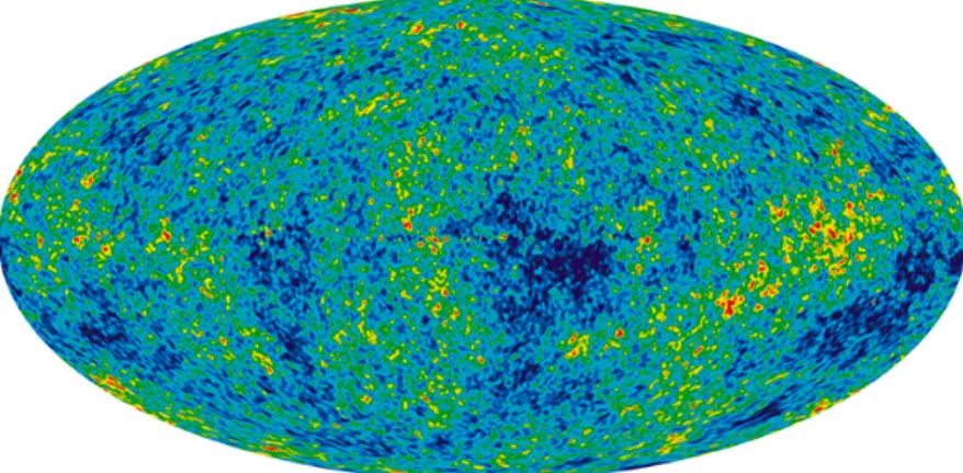
Fig. 1.5: WMAP-9yr result of CMB radiation. It shows the CMB temperature and fluctuation from -300µK (dark blue) to 300µK (red).

As the measurements have been improved, our knowledge of the universe has been pro- gressed. CMB has many kinds of physical information such as the Galaxy synchrotron and dust radiation (foreground radiation), lensing by the structure on large scales (sec- ondary), scattering by reionization, the CMB polarization, and gravity waves which are the main fluctuations generated in the early universe as predicted by an inflation theory.

Wilkinson Microwave Anisotropy Probe (WMAP) satellite (launched in 2001) measured CMB and its fluctuation in more detail. The small fluctuations are caused by the

(11)

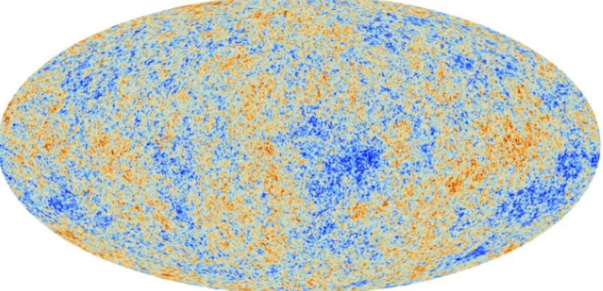
Fig. 1.6: CMB observed by Planck. It shows the temperature fluctuation in more detail from -300µK (blue) to 300µK (red). [10]

tiny density variations of the universe just after the Big Bang, the more a dense region tends to attract, the more matter results in a dense region. The process led to the formation of the first stars, galaxy and large scale structure. Planck satellite (launched in 2009) was the latest observation instrument. It has 2-3 times higher resolution compared to that of WMAP. It surveyed whole sky 5 times and finished the operation in 2014 (see Fig. 1.6).

Additional prediction is made by Zwicky in 1933, when he analyzed the relative motion between galaxies in the Comae Berenices. However, he could not explain why these galaxies are gravitationally bounded, contrary to the high speed of motion of galaxies.

There should be more than 100 times larger mass to be bounded in the cluster of galaxies.

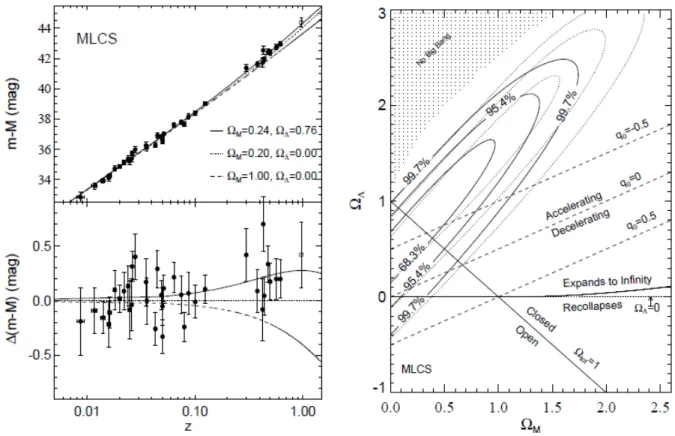
That is why they called this mass as ‘Missing Mass’, which could exist but we do not know the true character yet. Currently the Missing Mass is called dark matter. There is another fundamental prediction for Big Bang model. Riess et al. (1998) studied Hubble diagram (see Fig. 1.7) for type Ia supernovae. They revealed that the current universe is dominated by dark energy. It brought the current universe in the accelerated expansion epoch [11].

(12)

Fig. 1.7: Riesset al.determine the luminosity distance (including K−correction; redshift correction) via multi-color light curve shape (MLCS) method. The left-upper panel shows the Hubble diagram for type Ia supernovae samples. The best fit for a flat cosmology results in, Ω_M = 0.24, Ω_Λ= 0.76. The left-bottom panel indicates the diﬀerence between data and models with Ω_M = 0.20, Ω_Λ = 0, and the vertical line indicates empty universe with Ω_K = 1. The open symbol is SN 1997ck (z=0.97), which lacks spectropic classifi- cation and a color measurement. The right panel shows the (Ω_M,Ω_Λ) plane from type Ia supernovae. The solid contours are results from the MLCS method. The data of the dotted contours are the result excluding the unclassified SN 1997ck (z=0.97). This figure indicates that current universe is in the accelerated expansion phase. [11]

1.2 The Friedmann-Lema ˆı tre Model

The evolution of the universe is derived from the Einstein equation R_µν− 1

2g_µνR = 8πG (

T_µν− Λ 8πGg_µν

)

≡8πGT˜_µν, (1.1)

where g_µν is the metric tensor, T_µν is the energy momentum tensor, R_µν is the Ricci tensor, R is the scalar curvature, ˜T_µν is the energy momentum tensor including Λ-term as the dark energy, and G is the gravitational constant.

To solve (1.1) , we assume the following Cosmological Principle, and the fluid property:

(13)

• Universe is homogeneous and isotropic

ds² =dt²−a(t)²

[ dr²

1−kr² +r²(dθ²+ sin²θdϕ²) ]

. (1.2)

• Constituents can be regarded as the perfect fluid

T_µν = diag(ρ, P, P, P). (1.3)

Where, ρand P are the total energy density and the pressure,a(t) is the scale factor and k is the curvature constant. We take the unit system wherec= 1.

The left and right hand sides of the Einstein equation represent geometric structure of the space and the matter field. We can obtain an important equation from the conservation law ∇µT^µ0 = 0,

˙ ρ+ 3a˙

a(ρ+p) = 0, (1.4)

where the dot indicates ordinary derivative with respect to time. This equation describes density evolution. To solve (1.4), the equation of state (w =P/ρ) should be defined. In statistically thermal equilibrium, such thermodynamical variables are defined as follows;

n = g

∫ d³p

(2πℏ)³f(p) (1.5)

ρ = g

∫ d³p

(2πℏ)³E(p)f(p) (1.6)

P = g

∫ d³p (2πℏ)³

|p|²

3E(p)f(p) (1.7)

with use of Fermi-Dirac distribution function or Bose-Einstein distribution function (µ is the chemical potential);

f(p) = [

exp

(E(p)−µ k_BT

)

±1 ]₋₁

. (1.8)

The value of EoS w can be evaluated by using the above statistical quantitiesn and P. Here, n, p, E(p), g are number density, momentum, energy, internal degree of freedom,

(14)

respectively.

Notwithstanding these quantities, following definitions, are commonly used as the manner of cosmology;











w= 0 (For dust, matter component as the non-relativistic particles; ρ_m) w= 1/3 (For radiation as the (ultra) relativistic particles; ρ_γ)

w=−1 (For dark energy as the cosmological constant; ρ_Λ) The Einstein equation reduces to,

H² = (a˙

a )2

= 8πG 3

(

ρ+ Λ 8πG

)

− k

a², (1.9)

¨ a

a = −4πG

3 (ρ+ 3P), (1.10)

where H is the Hubble parameter. Energy density ρ consists of matter, radiation, and cosmological constant (ρ=ρ_m+ρ_γ+ρ_Λ).

Additionally, density parameters (Ω_i) are often defined using critical density at present ρcrit0 ≡3H₀²/8πG. Rewriting (1.9) using ρcrit0 and EoSw we get,

H² =H₀² (Ω_m0

a³ + Ω_γ0

a⁴ + Ω_k0

a² + Ω_Λ0 )

, (1.11)

or equivalently, H² =H₀²(

Ωm0(1 +z)³+ Ωγ0(1 +z)⁴ + Ωk0(1 +z)²+ ΩΛ0

), (1.12)

where Ω_i =ρ_i/ρ_crit is the energy density parameter and Ω_k =−k/H₀² is the density parameter for the curvature, the subscript 0 indicates that physical quantities are evaluated at the present epoch, z is the cosmological redshift (z = a0/a−1), respectively. The critical density parameter is

ρ_crit0 = 3H₀

8πG ≃1.88×10⁻²⁹h² g/cm³, (1.13)

wherehdefined ash=H₀/(100 km/s/Mpc) which is the dimensionless Hubble parameter.

By exploring the existence of the unique parameter set, we can check the correctness of Big Bang model and clarify how the universe evolves.

(15)

1.3 Big Bang Model and its Predictions

Big Bang model succeed in describing the evolution of the universe accurately. More- over, this theory predicts scientifically verifiable hypothesis, which has been remarkably consistent with many observations.

1.3.1 Big Bang Nucleosynthesis (BBN)

One of the most important successes of the Big Bang model is that primordial abundances of light elements can be quantitatively predicted. Light elements, such as D ³He,⁴He and

7Li, are synthesized in Big Bang nucleosynthesis (BBN). Big Bang nucleosynthesis is based on the simple assumptions of validity of Cosmological Principle. This theory predicts that light elements of D, ³He, ⁴He and⁷Li/H were synthesized during the first three minutes in the BBN epoch. BBN has good agreement with the primordial abundances which are estimated by observational data. Standard BBN model has the only one free parameter, baryon-to-photon ratioη =n_b/n_γ, where n_b and n_γ is the number density of baryon and photon. It is noted that the primordial value ofηdiﬀers from the present value ofηbecause of the electron-positron annihilation (see ‘Neutrino decoupling and pair annihilation’).

Before the electron-positron annihilation epoch, (11/4)η represents the baryon-to-photon ratio. The baryon density parameter is related to the density parameter Ω_b0;

η = n_b

n_γ = ρ_crit0

¯

mn_γ0 = 2.731×10⁻⁸Ω_b0h², (1.14)

where n_γ0 is the number density of CMB photons. We adopt the present temperature of the CMB photon of T_γ = 2.725 K [12, 13] and averaged mass ¯m = 1.675×10⁻²⁴ g which is adopted in Public Algorithm Evaluation the Nucleosynthesis of Primordial Elements (PArthENoPE) [14]. It is note that A. Coc precisely estimated the averaged mass ¯m[15];

¯

m = m_p(1−Y_p) + m_α 4 Y_p

= (1.6735−0.0119Y_p)×10⁻²⁴g,

where ¯m, m_p, m_α and Y_p are the averaged mass, proton mass, ⁴He mass and the mass fraction of ⁴He.

(16)

Thermal equilibrium epoch

At the high temperatureT_γ >3.0 MeV, neutrinos, neutrons, protons, electrons, positrons and photons are in the thermal equilibrium. This phase is dominated by the radiation component. The total energy density of radiation component (ρ_rad) is

ρ_rad =ρ_γ+ρ_e−+ρ_e⁺ +ρ_ν_e +ρ_¯_ν_e +ρ_ν_µ+ρ_¯_ν_µ+ρ_ν_τ +ρ_ν_¯_τ, (1.15) where each term of the right hand side indicates the energy density of photons, electrons, positrons, electron and anti-electron neutrinos, muon and anti-muon neutrinos, tauon and anti-tauon neutrinos, respectively. These energy components are estimated using (1.6) as

ρ_γ = 2·π² 30

(k_BT)⁴

(ℏc)³ ≡a_rT_γ⁴ (1.16)

ρ_ν = 7 8· π²

30

(k_BT)⁴ (ℏc)³ = 7

16a_rT_ν⁴ (1.17)

ρ_e = 7 8 2· π²

30

(k_BT)⁴ (ℏc)³ = 7

8a_rT_e⁴ (1.18)

wherea_ris the radiation constant (a_r =π²k_B/15ℏ³). Here, the scale factor dependence on the temperature can be written, ρ_γ ∝T⁴ ∝a⁻⁴. From the thermal equilibrium condition (T_γ =T_ν =T_e),

ρ_rad = (11

4 + 7 8N_ν^eﬀ

) a_r

(T_ν0 a

)4

, (1.19)

where N_νêff is the effective neutrino number and the standard theory of particle physics predictsN_νêff = 3.046 [16]. It includes the effects of (i) non-instantaneous neutrino decoupling and (ii) neutrino oscillations. T_ν0 is the present neutrino temperature.

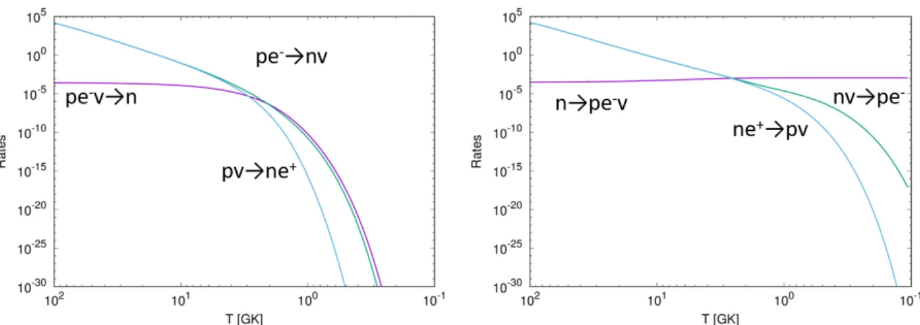
In addition, neutrons and protons are in the nuclear statistical equilibrium via weak interactions;

n←→p + e⁻+ ¯νe, (1.20)

n +ν_e ←→p + e⁻, (1.21)

n + e⁺ ←→p + ¯ν_e, (1.22)

(17)

where n, p, e⁻, e⁺, ν_e, ¯ν_e are neutrons, protons, electrons, positrons, electron neutorinos and anti-electron neutrinos, respectively.

The reaction rates for the weak interactions can be calculated as follows;

λ = σ(E)v_in

= 1

τ λ₀

∫ ( ∏

i:Lepton

4π p²_idpi

(2πℏ)³ f_i

) ( ∏

f:Lepton

4π p²_fdpf

(2πℏ)³ (1−f_f) )

δ(E_i−E_f), (1.23)

where, σ(E), v_in and τ are the scattering cross section and velocity of incident particle and lifetime of the specific nuclei. Here, p, f and E are the momentum and distribution function and total energy of leptons, and subscription ‘i’ (‘f’) denotes the initial (final) state of particles. Two termsδ(E_i−E_f) and (1−f_f) come from the energy conservation law and Fermi blocking factor.

The reaction rates corresponding to (1.23) are written in the following formulae [17];

λ_n_→_peν = 1 τ λ₀

∫ q 1

dϵ ϵ(ϵ−q)²(ϵ²−1)^1/2

[1 + exp(−ϵu)][1 + exp((ϵ−q)u_ν)], (1.24) λ_nν_→_pe = 1

τ λ₀

∫ _∞

q

dϵ ϵ(ϵ−q)²(ϵ²−1)^1/2

[1 + exp(−ϵu)][1 + exp((ϵ−q)u_ν)], (1.25) λ_ne_→_pν = 1

τ λ0

∫ _∞

1

dϵ ϵ(ϵ+q)²(ϵ²−1)^1/2

[1 + exp(ϵu)][1 + exp(−(ϵ+q)uν)], (1.26) λpeν→n = 1

τ λ₀

∫ q 1

dϵ ϵ(ϵ−q)²(ϵ²−1)^1/2

[1 + exp(ϵu)][1 + exp((q−ϵ)u_ν)], (1.27) λ_pe_→_nν = 1

τ λ₀

∫ _∞

q

dϵ ϵ(ϵ−q)²(ϵ²−1)^1/2

[1 + exp(ϵu)][1 + exp((q−ϵ)u_ν)], (1.28) λ_pν_→_ne = 1

τ λ₀

∫ _∞

1

dϵ ϵ(ϵ+q)²(ϵ²−1)^1/2

[1 + exp(−ϵu)][1 + exp((q+ϵ)u_ν)], (1.29) where τ is the neutron lifetime, u= m_e/T_γ, u_ν =m_e/T_ν, ϵ =E_e/m_e, q = ∆m_np/m_e. λ₀ is definded as

λ₀ =

∫ _q

1

dϵ ϵ(ϵ−q)²(ϵ²−1)^1/2 ≃1.63609, (1.30) where it is defined to satisfy λ_n→peν → τ⁻¹ when T_γ → 0 and T_ν → 0. In other words, it is introduced to adjust λn→peν to the experimental value of neutron lifetime at the low temperature (see Fig. 1.8). On the other hand, the other reaction rates converge toλ→0.

(18)

Fig. 1.8: The relation between reaction ratesλ and the photon temperature T.

Neutrino decoupling and pair annihilation

When the temperature drops toT_γ ≃1.5 MeV, weak interactions freeze out and neutrinos decouple from the other particles. After the neutrino decoupling, neutrinos behaves free particles and the momentum distribution conserves by themselves. Then the temperature drops toTγ ≃0.7 MeV, electron-positron annihilation begins via the following reaction:

e⁺+ e⁻ −→γ+γ.

Energy from electron-positron pairs flows in photons via pair annihilation. The annihilation is completed at T_γ ≃ 0.4 MeV. At this epoch, the total energy density of radiation component becomes

ρ_rad =ρ_γ+ρ_ν_e +ρ_ν_¯_e+ρ_ν_µ +ρ_ν_¯_µ+ρ_ν_τ +ρ_ν_¯_τ. (1.31) To estimate the temperature evolution of photons and neutrinos, entropy conservation law is used. The entropy s(a, T) is defined as follows,

S(a, T)

V ≡s(a, T)≡ ∑

i:particle

1

T_i (ρ_i+P_i). (1.32)

(19)

Where the entropy per unit co-moving volume is conserved because of its independency from the cosmic expansion. In this situation, electron and positron should not be treated as relativistic particles, that is, entropy of electron-positron pairs are evaluated using (1.6) and (1.7);

s_e(a, T_γ) = 1

T_γ(ρ_e+P_e)

= 1

T_γ

g_e−+g_e⁺ (2π)³

∫ _∞

0

dp_e [

4πp²_e(√

m²_e+p²_e+ 1 3

p²_e E_e

) 1

1 + exp(E_e/k_BT_γ) ]

= 1

T_γ 2

π²(k_BT_γ)⁴ Se

( me

k_BT_γ )

(1.33) where, g_i is the internal degree of freedom, E =√

m²_e+p², and we defineSe as Se(x)≡

∫ _∞

0

y²dy (√

x²+y²+ 1 3

y²

√x²+y² )

1 1 + exp(√

x²+y²). (1.34) We have to consider conservation law only for photons and electron-positron pairs since they are interacting suﬃciently;

s = 4 3a_rT_γ³

[ 1 +

(4 3a_rT_γ³

)₋1

· 1 T_γ

2

π²(k_BT_γ)⁴Se

]

= 4 3a_rT_γ³

[

1 + 45 2π⁴Se

]

= 4 3a_rT_γ³J

( m_e kBTγ

)

(1.35) J(x), which is the entropy of photons plus electron-positron pairs in unit of entropy of the photons, is defined as,

J(x) ≡ 1 + 45

2π⁴Se(x). (1.36)

Adopting (1.35) and conservation law (1.32) for before and after the pair annihilation

(20)

period, we obtain the following relations;

s_bef =s_aft

⇐⇒ 11

3 a_rT_bef³ = 4

3a_rT_aft³J

⇐⇒ 11

3 a_rT_ν³ = 4

3a_rT_γ³J

⇐⇒ T_ν = ( 4

11 )1/3

T_γ [

J ( m_e

k_BT )]1/3

(1.37)

Fig. 1.9: Photon (Tγ) and neutrino (Tν) temperature evolution.

If massless neutrinos completely decoupled from photons, the neutrino temperature T_ν always proportional to the inverse of the scale factora⁻¹ (see Fig. 1.9). The subscripts

’bef’ and ’aft’ indicate the entropy of before electron-positron pair annihilation and after the annihilation, respectively. It is noted that the neutrino temperature in the reaction rates (1.24)-(1.29) should be estimated using the relations during this period.

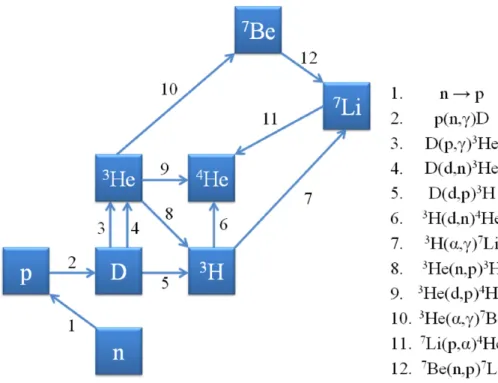
Light elements synthesis

When the temperature falls toT_γ ≃0.1 MeV, light element synthesis begins (see Fig. 1.10).

(21)

Fig. 1.10: The most important reaction network for Big Bang nucleosynthesis.

1.3.2 Observation of light elements

Helium-4

We show the [O/H]-Y(⁴He) plane and the variations for observational values in Fig. 1.11.

The blue points with error bars represent the abundance in the HII region. The solid curve indicates the most probable path obrained from the chemical evolution calculation. The primordial abundance of ⁴He is obtained by taking the limit of [O/H]= 0. Observational values in recent years tend to have the consistency with the BBN calculation results.

Helium-4 that exists in the universe is mostly synthesized during BBN, but in the star’s evolution process. Hydrogen is burned by p-p chain in the deeper region, and ⁴He is synthesized. Therefore, these quantities are included in the observational values, in the Low-z region where the heavy elements are small. If the element synthesis inside the star is not active, the composition of ⁴He produced by BBN remains as it is. Therefore, estimation of ⁴He has been done from direct observation of ⁴He or recombination line of hydrogen in the HII region outside the galaxy with small amount of metal. However, the estimation of ⁴He in the HII region outside galaxy involves indeterminacy due to the

(22)

uncertainty of the observation and the complexity of the physical process in the HII region.

For example, it is diﬃcult to measure the temperature, electron density and optical depth of the region.

Fig. 1.11: Left: Estimation of the primordial abundane of ⁴He [18]. Right: Changes in observed values of Helium-4 [19].

Deuterium

Since the composition ratio of deuteron strongly depends on baryon-to-photon ratio η, it is an element also called ‘baryometer’. Deuteron is synthesized only in the early universe during BBN, it can be considered to decrease due to the destructive reaction inside the stars (D(p,γ)³He). Therefore, D+³He has been considered to give the upper limit of deuteron. However, the generation process of ³He in the star is not known in detail, and its evaluation is diﬃcult. Therefore, the composition of deuteron is currently estimated by observing the absorption line from QSO at high redshift. Since QSO is a primitive galaxy at the beginning of galaxy formation, it can be a source of information for early universe.

We show the chemical evolution of deuteron in the left panel of Fig. 1.12. The solid red curve is calculated using the Times code [20]. We input the BBN production of deuteron since the low metallicity region ([O/H]< −1.5) reflects the BBN production. During the evolution of galaxies, deuteron has been destructed and its abundance decrease. It indicates that the observational value at the region of [O/H]<−1.5 is compatible with the BBN production. The right panel in Fig. 1.12 shows the wide absorption line of hydrogen

(23)

and deuteron. The sharp absorption line (∼4907˚A at the upper panel) represents the line of Si_IIIλ 1206.5, which is used to estimate the redshift of the absorption line from QSO.

Fig. 1.12: Left: Chemical evolution of deuterium. Right: Absorption lines [21].

Lithium-7

The observation of ⁷Li/H is carried out for the halo stars of the population III with a small amount of metal. ⁷Li is burned in the evolution process of the star and its amount decreases; in older galaxies with a small amount of metal, it includes the early universe of BBN. It is estimated that the generated⁷Li remains. ⁷Li/H has been observed since ‘Spite plateau’ was predicted on the [⁷Li/H]-[Fe/H] plane. The primordial value is obtained by calculating the ⁷Li value of zero metalicity on the [⁷Li/H]-[Fe/H] plane after considering the depletion of ⁷Li in the observation data. In Fig. 1.13, the green curve is calculated using the Times code [20], and the blue and red points with error bars are the estimated value of ⁷Li for each star. The purple and dark green points indicate the averaged values in 28 dwarfs (Sbordone et al.), and in 18 dwarfs (Korn et al.). Korn et al. consider the significant depletion and/or destruction for ⁷Li abundance during the lifetime of Population II stars.

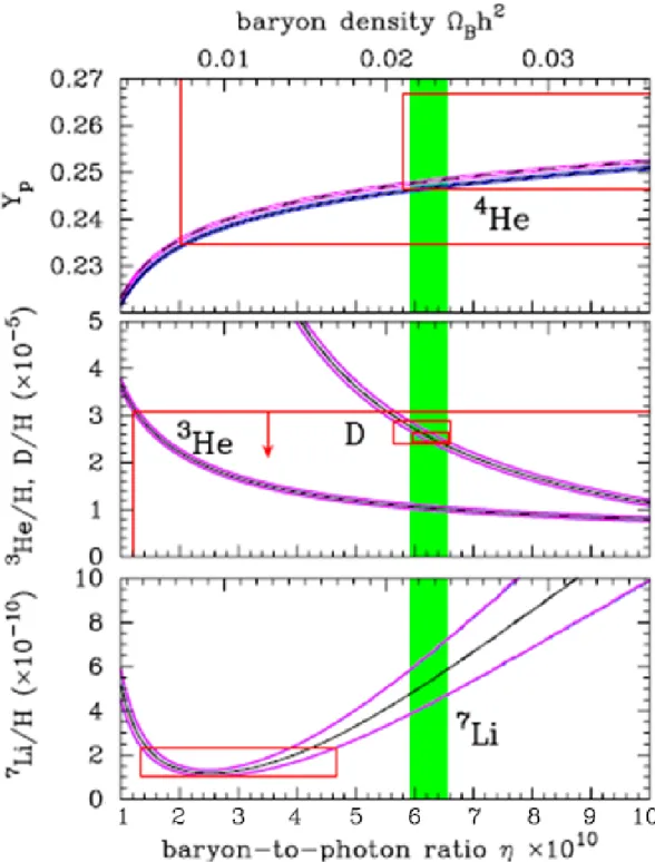
In Fig. 1.14 the observational results of ⁴He and D, and BBN results are consistent with CMB constraints on baryon-to-photon ratio or baryon density. In addition, ⁴He and D results give the reasonable extent for the baryon density.

(24)

Fig. 1.13: Chemical evolution of lithium-7 and its observational values [19].

(25)

Fig. 1.14: The black curves indicate that abundance of light elements, ⁴He(Y_p), D, ³He and ⁷Li which are predicted by the standard Big Bang nucleosynthesis. Blue lines are calculated with neutron lifetime τn = 878.5±0.8 s and purple lines are calculated with τ_n = 885.7±0.8 s. And these lines are including uncertainties of reaction rates. Red boxes show the 2σ errors of observational prediction and the vertical lines come from the constraints on baryon density. The green vertical band indicates the constrains on baryon density from WMAP [22].

(26)

1.3.3 Magnitude-redshift relation

The key idea of the precise measurements of the magnitude-redshift relation (m − z relation) is to adopt the distance ladder. It is the sequential method in determining the distance from the earth to astrophysical objects. A direct measurement is possible only for those objects that are close enough to observer. The techniques in determining distances are based on various correlations in stellar objects. Several measurements rely on a standard candle, such as type Ia supernovae, which has a known luminosity. At present, there is no unified method to measure the distance for distant objects. It is necessary to measure the distance of the nearby object in some method, and then referencing it and obtains the distance of more distant objects. This process is called ‘distance ladder’.

Hence, m−z relation plays a key role in determining the cosmological parameters.

The cosmological distance measurements or estimations, concerning with the magnitude, enormously depend on the cosmological redshift, curvature, density parameters and Hub- ble parameter. Distance is measured by the luminosity of stellar objects such as Cepheid variables and type Ia supernova. These objects are known as the standard candle. Addi- tionally recent study makes it possible to use gamma-ray bursts as the standard candle.

The quantity of the distance, which is measured by the luminosity, is called luminosity distance (d_L). This quantity is aﬀected by cosmological redshift directly and the spectrum is shifted. The redshift is caused by the expansion of the universe, so that the relation between magnitude and redshift (m−z relation) is one of the most important observational quantity to evaluate how the universe evolves.

1.3.4 Measurements of magnitude-redshift relation

Cepheid variables

The stars outside the Galaxy are dark and it is diﬃcult to measure the spectrum and luminosity. We need to explore the bright stars what we can observe. In Magellanic nebulae, bright stars are found which changes the luminosity periodically from 10³L_⊙ to 10⁶L_⊙. These stars are called ‘Cepheid variables’ and the period is about 1∼135 days.

It changes the luminosity because of their expansion and contraction in the envelope.

Moreover, it is discovered that the longer the period of logP, the brighter the absolute magnitudeM (see Fig. 1.15). Using the relation between period and absolute magnitude,

(27)

Fig. 1.15: Correlation between period and absolute magnitude (luminosity) of Cepheid variables [23]. Since we can obtain the absolute magnitude from the period, we estimate the distance to the star, which becomes the first ‘ladder’.

the distance of more distant Cepheid can be estimated.

Type Ia supernova

There is a popular phenomenon called supernova explosion. There are many kinds of type for supernova explosions, such as type Ia, type Ib, type Ic and, type II supernovae.

In particular, type Ia supernova has luminosity about 10¹²L_⊙, and the luminosity only slightly depends on indivisual stars. Moreover, it is discovered that there is a relation between the peak luminosity MB and the change rate of the luminosity after 15 days

∆m₁₅. This relation is called M −∆m₁₅ relation or Phillips relation (see Fig. 1.16).

Many observational results have been accumulated using this relation. Therefore, the compilation data are available up to the redshift z ∼1.5 for type Ia supernovae.

(28)

Fig. 1.16: Left: Correlation between magnitude and ∆m₁₅ of type Ia supernova [24].

Right: Correction of the light curve of type Ia supernovae by redshift and Phillip relation [25].

Gamma ray burst

Gamma ray burst is the brightest celestial phenomenon and the luminosity is reached to 10²⁰L_⊙. There are two candidates of gamma ray bursts: gravitational collapse of star and neutron stars merger. However, the mechanism is not well understood. Recently, the gamma ray bursts have been enthusiastically studied [26–29] and it gradually turned out that gamma ray bursts have some features on their own. For instance, Amati relation represents the relation between the isotropic energy and peak energy [27, 28].

(29)

1.4 Problems in the Present Cosmology

Recent observations indicate that our universe is flat and has turned into accelerated expansion phase at the present epoch [11, 30–33]. Some cosmological models have been introduced to examine the characteristics of the present acceleration [34–39]. The most simple one is the ΛCDM model, which includes Λ term as a dark energy. The Λ term leads to the negative pressure, and moderate the universe for acceleration. This is the standard model of the present cosmology having a dark sector which consists of dark energy and dark matter. Dark matter and dark energy should be around 25% and 70% at the present epoch, respectively [30].

Up to now, the ΛCDM model is almost consistent with many observations of CMB and SN Ia [31, 40], with the exception of the typical estimations of the vacuum energy which are many orders larger than the observed one [41]. Recently, many observational results have been accumulated about SN Ia. Therefore, the compilation data are available up to the redshift z ∼1.5. We have a great interest of investigating the feature of dark energy (DE) around small redshift region. While CMB includes the area of very large redshift compared to the one of SNe Ia, we may have to interpolate the behavior between them if we study DE quantitatively. As a consequence, the data z ≥1.5 would become important to constrain the behavior of DE in a wide range of cosmological epoch.

Recently, the GRBs have been enthusiastically studied [26–29] to investigate the behavior of DE and the expansion rate at high redshift range. As a consequence, we can discuss the density evolution of DE in detail.

Clarifying the properties of DE is one of the most important issues in cosmology, and especially modifying an EoS and/or a gravitational field is the most popular method.

Although these are methods to represent the features of DE, it is presumed that DE belongs to dynamical phenomena. Some theoretical dark energy models have been proposed to describe the energy density evolution. For instance, models of quintessence, phantom, quintom, k-essence, Chaplygin gas and so on, belong to non-standard DE models [34–38, 42]. On the other hand, some models which include the modified EoS of dark energy give more direct method. We can categorize above models as follows: (i) Cosmo- logical constant (w=−1). (ii) DE with constant but w ̸=−1. (iii) Dynamical DE with w > −1 (Quintessence-like models). (iv) Dynamical DE with w < −1 (Phantom-like

(30)

models). (v) Dynamical DE which crosses the phantom barrier of w = −1 (Crossing models).

Recent observational results indicate that EoS of DE accrosses the barrier of w=−1, so called phantom barrier [43–46]. Some theoretical models, which accross the phantom divide, have been extensively studied [47,48]. On the other hand, a modified EoS is easier to handle the density evolution of DE, and it is beneficial to understand the asymptotic behaviour of DE to examine whether the crossing exists or not.

In the present work, we investigate how DE should be categorized by modifying the EoS directly. We adopt a special EoS whose functional form has two limiting values of parameters. In addition, with use of the observational results such as SN Ia and gamma- ray burst (GRB), we constrain specific parameters in EoS of DE over a wide range of the redshift around 1<(z+ 1)<10.

Big Bang nuleosynthesis provides substantial clues for investigating physical conditions in the early universe. Standard BBN produces about 25% of the mass of the Universe in the form of ⁴He, which has been considered to be in good agreement with its observed abundance in a variety of astronomical objects.

The produced amount of⁴He depends strongly on a fraction of neutrons at the onset of nucleosynthesis, but is not very sensitive to the baryon-to-photon ratioη(η=n_b/n_γ;η₁₀ = 10¹⁰η). Hence the produced amount of ⁴He is used to explore the expansion rate during BBN, which ca be related to the eﬀective number of neutrino flavors. In addition to

4He, significant amounts of D, ³He, and ⁷Li are also produced. Because of its strong dependence on η, the abundance of D is crucial in determining η and consequently the density parameter of baryons Ω_b.

In spite of the apparent success of standard BBN (SBBN), recent observed light elements, which are considered to be primordial, have been controversial. Large discrepan- cies for⁴He observations emerge between diﬀerent observers and modelers of observations:

rather high values of ⁴He have been reported for H II regions in blue compact galaxies.

It is noted that the primordial abundance of ⁴He is deduced from extrapolation to zero metallicity. The deuterium abundance has been observed in absorption systems toward high -redshift quasars. It should be noted that the value of D has been believed to limit the present baryon density. A low value of ⁷Li observed in Population II stars reported by Bonifacio et al. is considered to be due to depletion and/or destruction during the

(31)

lifetimes of stars from a high primordial value.

Recently, the lifetime of neutrons has been updated from the previous adopted value of 885.7 ± 0.8 s which has been used commonly in BBN calculations consistent with the observed abundances of ⁴He and D. However, the latest compilation by Beringer et al.

determined the mean life to be 880.1±1.1 s, which may suggest an inconsistency between BBN and observational values. This indicates a further inconsistency with theη deduced byPlanck.

The apparent spread in the observed abundances of ⁴He should give rise to an incon- sistent range of η. Apart from observational uncertainties, we have no reliable theories beyond the standard theory of elementary particle physics. It is assumed in standard BBN that there are three flavors of massless neutrinos which are not degenerate. How- ever it was suggested by Harvey and Kolb that lepton asymmetry could be large even when baryon asymmetry is small. The magnitude of the lepton asymmetry is of particular interest in cosmology and particle physics. Related to neutrino oscillations, investigations of BBN have been revised with the use of nonstandard models. As presented by Wagoner et al.and Beaudet and Goret, the abundances of light elements are modified by neutrino degeneracy; it could be necessary and crucial to search consistent regions in η within a framework of BBN with degenerate neutrinos by comparing it with the latest observation of the abundances of ⁴He and D.

If neutrinos are degenerate, the excess density of neutrinos causes speedup in the expansion of the Universe, leaving more neutrons and eventually leading to enhanced production of ⁴He. On the other hand, degenerate electron neutrinos shiftβ equilibrium to less or more neutrons and hence change the abundance production of ⁴He. The latter eﬀect is more significant than the former. In the present paper we investigate BBN by including degenerate neutrinos and using up-to-date nuclear data. Referring to several sets of combinations for recent observed abundances of ⁴He and D, we derive consistent constraints between η and the degeneracy parameter.

(32)

2 Big Bang Nucleosynthesis

2.1 Observed Abundance of Light Elements

There exist very large spreads in some observed abundances of light elements due to diﬀerent observational methods. Let us describe how we adopt the observed primordial abundances. The primordial abundance of ⁴He can be measured from observations of the helium and hydrogen emission lines from low-metallicity blue compact dwarf galaxies. Izotov et al. reported the ⁴He abundance from a subsample of 111 HII regions as follows [49]:

Y_p = 0.254±0.003. (2.1)

The observational value of ⁴He has large uncertainty, because the abundance could be appreciated to having the zero metallicitiy in terms of an extrapolation by a model of the chemical evolution of galaxies. An alternative low value of the average was reported by Averet al. [50]

Y_p = 0.2464±0.0097, (2.2)

which has a very large spread in errors.

Deuterium is the most crucial element to determineηbecause of the strong and mono- tonic dependence on η. Its primordial abundance is determined from metal-poor absorp- tion systems toward high-redshift quasars. Cooke et al. have performed measurements at redshift z = 3.06726 toward QSO SDSS J1358+6522 [21]. Additionally, they have analyzed all of the known deuterium absorption-line systems that satisfy a set of strict criteria,

D/H = (2.53±0.04)×10⁻⁵. (2.3)

This value corresponds to the baryon density Ωbh² = 0.02202±0.00046 which is consistent with the results of thePlanckobservation. Here his the Hubbule constant in units of 100

(33)

km/s/Mpc.

We should note that the observed abundance of ⁷Li in Population II stars is given by Sbordone et al. [51] to be

7Li/H = (1.58±0.31)×10⁻⁸, (2.4)

which has been advocated to be rather low compared with BBN. While considering significant depletion and/or destruction during the lifetimes of Population II stars, Korn et al. derived a high primordial abundance, [52]

7Li/H = (2.75−4.17)×10⁻¹⁰, (2.5)

the value which is still too low to be reconciled with the result of BBN. It is noted that Li can be produced together with Be and B through spallation of CNO nuclei by cosmic ray protons and α particles. About 10% of ⁷Li could be due to cosmic-ray processes, leaving the remainder as primordial. Among a variety of observational data, we here pick up only representatives of ⁴He and D.

2.2 Standard BBN and Reaction Rates

In general, reaction rate is averaged by Maxwell-Boltzmann distribution;

N_A⟨σv⟩=N_A

( 8 πµk³_BT_γ³

)1/2∫ _∞

0

σ(E)Eexp (

− E k_BT_γ

) dE,

where N_A, v, σ and µ are the Avogadro number, relative velocity, cross section and reduced mass. The reaction cross section of charged particle are shown as

σ(E) = S(E) exp(−2πζ)

E ,

where S(E) is the S-factor, and ζ is the Sommerfeld parameter which is given by the following formula;

ζ =Z₁Z₂ (e²

ℏc

) (µc² 2E

)1/2

,

(34)

here, Z_i is the charge in unit of elementary chargee. On the contrary, the reaction cross section with neutrons is

σ(E) = R(E) v ,

where R(E) is the transition probability and v is the velocity of incident particle.

2.2.1 Latest obsrvational data and BBN calculation

First of all, twelve reactions and corresponding literature, which greatly influence the final production amount of elements in BBN, are shown in Table 2.1. We performed BBN calculation with use of BBN code (Hashimoto and Arai [53]). All reactions are given in Appendix A(Table A.2).

Table 2.1: BBN main paths and the references.

1 n↔ p (1.24)-(1.29) 7 T(d,n)⁴He DE04 2 p(n,γ)D An06 8 ³He(d,p)⁴He DE04 3 ³He(n,p)T DE04 9 ⁷Li(p,α)⁴He DE04 4 D(p,γ)³He DE04 10 T(α,γ)⁷Li DE04 5 D(d,n)³He DE04 11 ³He(α,γ)⁷Be DE04 6 D(d,p)T DE04 12 ⁷Be(n,p)⁷Li DE04

We apply DE04 [54] for reaction network, which are the nuclear reaction rates derived using theR-matrix analysis. It has been recommended conventionally for the main paths of nucleosynthesis. We adopt 880.1±1.1 s [55] for neutron lifetime, which is one of the most important physical quantity and enormously aﬀects the⁴He abundance.

In Fig. 2.1, we show the main result of standard Big Bang nucleosynthesis with use of DE04 [54]. From the top panel, the figure shows the⁴He mass fraction (Yp) and number fraction of deuteron and ⁷Li comparison to proton (H).

Figure 2.1 indicates three points,

• Lithium problem still remains as the serious problem.

• The result of Izotov (2013) is consistent with that of Aver (2013), but is not consistent with observational result of deuteron by Cooke (2014) and Planck 2013 [56].

• BBN result has no answer for the baryon-to-photon ratio using the results of (2.1) and (2.3).

(35)

Fig. 2.1: Dependence of light elements abundances on η₁₀ using DE04 [54] reaction rates. We apply τ_n = 880.1 for the neutron lifetime [55]. Vertical band is the constraints on baryon-to-photon ratio from P lanck 2013 [56]. Indivisual error bands indicate 2σ confidence level.

We focus on the last two problems because they are the more serious problem than the lithium problem. As the first step of the improvement, we adopted the nuclear reaction rate of NACRE-II compiled by incorporating the experiment result of recent years, and BBN calculation was carried out considering the uncertainties in nuclear reaction rates. We apply NACRE-II for D(p,γ)³He, D(d,n)³He, D(d,p)T, T(d,n)⁴He,³He(d,p)⁴He,

7Li(p,α)⁴He, T(α,γ)⁷Li and ³He(α,γ)⁷Be, respectively. The results are shown in Fig. 2.2 and Table 2.2.

Table 2.3 is the result of calculation using η = 6.19×10⁻¹⁰. It indicates that the reaction paths significantly aﬀects abundances. At first, let us discuss the final abundances of deuteron and ⁷Li. Compared to the reaction rate of DE04, NACRE-II reaction rate consumes deuteron−2.3% via D(d,p)T. D(p,γ)³He has the opposite tendency which causes an increase of deuteron by +0.7%. Together with these two reactions, NACRE-II reaction rates have the tendency of consuming more deuterons. NACRE-II reaction rate has the tendency of producing more ⁷Li via D(p,γ)³He(α,γ)⁷Be(,e⁺νe)⁷Li.

(36)

Focusing on the box of D/H, the result using NACRE-II is smaller in error with the observed value of P lanck 2013 than in the case of using DE04, resulting in a more consistent result. Also, when determiningη10 from⁴He, we obtain the small diﬀerence of the baryon-to-photon ratio δη₁₀ ∼ −0.07. Therefore, the influence of nuclear reaction rate [54] and [57] is not so large. It is reasonable to evaluate the results of BBN using only the value of η₁₀ obtained from D and the nuclear reaction rate of NACRE-II, which are consistent with P lanck satellite.

Fig. 2.2: η dependency of light elements abundances using NACRE-II reaction rates. We apply τn = 880.1 s for the neutron lifetime. Vertical band is the constraints on baryon- to-photon ratio fromP lanck 2013. Each error bars indicate 2σ confidence level.

Table 2.2: Constraints on η₁₀ from ⁴He and D observation using DE04 and NACRE-II.

DE04 NACRE-II observation

D η₁₀= 6.08−6.54 η₁₀= 5.99−6.48 Cooke+ 2013 Y_p η₁₀ ≥6.77 η₁₀ ≥6.70 Izotov+ 2013 Yp η10 ≥2.33 η10 ≥2.31 Aver+ 2013