1. Introduction
Synoptic current fluctuations having typical temporal scales of weeks to months and horizon-tal scales of tens to hundreds of kilometers are called “mesoscale eddies.” They are also called “low-frequency fluctuations” or “low-frequency eddies.” Mesoscale eddies dominate in the mid-ocean flow field(ROBINSON, 1983). They were first recognized from observations in 1959 by neutrally-buoyant floats at mid-depths in the North Atlantic(CREASE, 1962).They have been measured by moored current-meters and
neu-trally-buoyant floats at depth, most intensively in 1970s and 1980s. The highlight was the Mid-Ocean Dynamics Experiment(MODE)carried out in 1973 in the western North Atlantic (MODE GROUP, 1978). Mesoscale eddies at sur-face layers have been measured by sursur-face drifting-buoys tracked by satellites(NIILER, 2001). Since the Topex/Poseidon satellite was launched in 1992, mesoscale eddies have been intensively measured by satellite altimeters; details of meso-scale eddies with surface manifestation have been revealed, especially for their global views (FUand MORROW, 2013).
To understand the nature of mesoscale eddies, their mechanisms and their roles in ocean circu-lation, observations at depth are necessary as well as surface observations. A considerable
Mesoscale eddies observed by moored current-meters at abyssal
depths in the western North Pacific during 1978Ȃ1985
Shiro IMAWAKI1)*and Kenzo TAKANO2)
Abstract: Observations by moored current-meters were carried out repeatedly in mid-ocean of the western North Pacific, providing 50 velocity records. A continuous velocity record for al-most seven years was obtained at 5000 m depth. The overall mean velocity is directed to the north with a speed of less than 1 cm s-1. The kinetic energy of low-frequency
velocity-fluctuations, or mesoscale eddies is more than 30 times larger than that of mean flow. Frequen-cy spectra of eddy kinetic energy show that most of the energy is contained in mesoscale bands (periods of 31Ȃ235 days),with zonal(meridional)dominance of energy in the longer(shorter)
period band. An array observation at 4000 m depth shows that the local change of relative vor-ticity of mesoscale eddies is balanced mainly with the advection of planetary vorvor-ticity, although the horizontal advection of relative vorticity and higher-order horizontal divergence may play some role. Those results suggest that the mesoscale eddies are understood as primarily plane barotropic Rossby waves with possible modification.
Keywords : mesoscale eddies, moored current-meter, frequency spectrum, vorticity balance
1)Professor Emeritus of Kyushu University, Yoko-hama, 224Ȃ0014, Japan
2)Matsudo, Chiba Prefecture, 271Ȃ0064, Japan *Corresponding author:
E-mail: [email protected]
1)Institute of Marine Science, Burapha University, Bangsaen, Chon Buri 20131, Thailand
2)Department of Aquatic Science, Faculty of Sci-ence, Burapha University, Bangsaen, Chon Buri 20131, Thailand
3)Atmosphere and Ocean Research Institute, The
University of Tokyo, 5Ȃ1Ȃ5, Kashiwanoha, Kashi-wa, Chiba 277Ȃ8564, Japan
*Corresponding author: Thidarat Noiraksar Tel: + 66(0)38 391671
Fax: + 66(0)38 391674
fraction of velocity and temperature fluctuations observed in the MODE area is accounted for by a combination of barotropic and first-mode baro-clinic Rossby waves(MCWILLIAMS and FLIERL, 1976).In the Gulf Stream recirculation region in the North Atlantic, a barotropic Rossby wave modified by bottom topography was observed beneath the thermocline(PRICE and ROSSBY, 1982).At a site called R to the east of the Izu-Ogasawara Ridge in the western North Pacific, a considerable fraction of mesoscale eddies at abyssal depths is accounted for by a set of three barotropic Rossby waves(IMAWAKI, 1985). Re-cent studies show that fluctuations at the same site having specific spectral peaks are explained by plane topographic Rossby waves(MIYAMOTO et al., 2017; 2019).Under the Kuroshio Extension, topographic Rossby waves in a period band of 30Ȃ60 days were observed(GREENEet al., 2012). Examination of vorticity balance of mesoscale eddies at 1500 m depth in the MODE area shows that a 10Ȃday mean balance is highly nonlinear but a 60Ȃday mean balance is marginally linear (MCWILLIAMS, 1976). In the North Equatorial Current region in the Atlantic, the local change of relative vorticity is balanced with the advec-tion of planetary vorticity in the thermocline as well as in the deep layer, for a period band of 24Ȃ81 days(KEFFER, 1983).At the Site R to the east of the Izu-Ogasawara Ridge, the local change of relative vorticity is accounted for by the advection of planetary vorticity at 5000 m depth within the estimated error(IMAWAKI, 1983).
These studies suggest that the dynamics of mid-ocean mesoscale eddies differs at locations, depths and temporal/spatial scales, and further examinations are required to understand the ed-dy field. Intensive observations by moored cur-rent-meters were carried out at abyssal depths at more than 20 stations in the Site R during
1978Ȃ1985, in order to primarily investigate mes-oscale eddies. The present paper provides de-scription of the velocity measurements and re-sults obtained mostly on mesoscale eddies.
The rest of the paper is organized as follows. Section 2 describes the observation site, mooring operations, current measurements and data processing. Section 3 gives general statistics of individual velocity records and describes com-bining individual records. Section 4 shows fea-tures of mean flows. Section 5 describes statisti-cal features of mesosstatisti-cale eddies. Section 6 shows features of frequency spectra. Section 7 de-scribes the vorticity balance of mesoscale eddies using the current-meter data, with Subsection 7.1 on Array-83 and Subsection 7.2 on Array-84. Sections 8 and 9 are discussions and summary, respectively.
2. Current measurements
The observation site called R is centered at 30°N, 147°E in the western North Pacific. At shallow depths, the site center is located about 400 km south of the Kuroshio Extension(Fig. 1) and on the indistinct southern boundary of the broad west-southwestward flowing Kuroshio Countercurrent(UCHIDA and IMAWAKI, 2003).At abyssal depths, it is sufficiently distant from the weak deep western boundary current located east of the Izu-Ogasawara Ridge(KAWABE and FUJIO, 2010).Like the MODE area, the observa-tion site is located between a strong current re-gion and the interior.
Figure 1 also shows bottom topography based on ETOPO1(AMANTE and EAKINS, 2009). The site center is located about 500 km east of the Izu-Ogasawara Ridge. The water depth varies between 6000 and 6300 m within 100 km of the center. The bottom topography is generally flat with small gentle undulations and no apparent large-scale slopes. Exception is several
sea-mounts, for example, a small seamount near Stn. RR, which was not known at the observation time.
Configuration of a used conventional inter-mediate mooring is shown in Fig. 2 schematical-ly. The mooring line with current-meters insert-ed was designinsert-ed to be held vertical in fluctuating flows by both large buoyancy of a glass-sphere cluster at the top and dead weight on the sea-bed. The mooring was deployed by the so-called “buoy-first/anchor-last” way. It was recovered by releasing an anchor weight through a com-mand from the ship to an acoustic release. When
the mooring line surfaced, a radio-transmitter sent a radio signal to the ship to be located. The mooring technology had been developed by the Buoy Group of Woods Hole Oceanographic Insti-tution(HEINMILLER, 1976)and was transferred to Japan in mid 1970s.
Numbers of current-meters were moored mostly at abyssal depths at various locations in Site R(Fig. 1)repeatedly during 1978 through 1985. Table 1 shows the summary of mooring op-erations. First moorings were deployed in Octo-ber 1978. In March 1979, they were recovered and second moorings were deployed on the same Fig. 1 Location of mooring stations with bottom topography. Dots with station names show
lo-cations where current-meter data were obtained; the first “R” of station names is omitted. Two open circles show locations where moorings were deployed but not recovered in Obs. 9. Darker gray indicates shallower depth, with contours of 500 m interval. The rectangle within the small-scale physiographic inset illustrates the location of the present study area relative to both the Kuroshio system, whose mean path during 1993Ȃ2000 is shown by shading, and the Izu-Ogasawara Ridge, whose horizontal extent at 3000 m depth is shown by dotted lines.
cruise. Such recovery and deployment cruises were repeated. Finally, last moorings were re-covered in July 1985. As a result, nine mooring observations were performed; they are called Obs. 1 through 9.
Totally 44 moorings were deployed. Thirty-two of them were recovered successfully to pro-vide numbers of good quality records. Two oth-ers were recovered without useful records. Ten were not recovered, mostly in Obs. 3, probably because anchor weights made of bundling cut-rails were taken apart during mooring. There-fore, the recovery rate of mooring is 77 % as a whole; it increases to 87 % if Obs. 3 is excluded. Data were not retrieved successfully from 13 current-meters on 12 recovered moorings; they are not listed in Table 1. Totally 50 records are
available. Measurements were restricted mostly to abyssal depths because our mooring technolo-gy at that time did not allow us to obtain safe and stable platforms at shallow depths.
Aanderaa RCM-5 current-meters were moor-ed. The current-meter measured current speed by a Savonius rotor and current direction by a magnetic compass, which detected the direction of the instrument body following the fluctuating flow freely. The current-meter recorded current speed, current direction and temperature on a small magnetic tape at an interval of mostly one hour.
After the recovery, the data were linearly in-terpolated in time, in order to correct possible gain or delay of the inside clock and provide the data every hour on the hour, if recording had continued until the recovery; the discrepancy was typically less than one hour. The reference of flow direction was transferred from the mag-netic north to the true north; the magmag-netic north was located to 2Ȃ3°W at the present site. Then noises and doubtful data were removed by eye.
An example of raw data from a nominal depth of 4000 m is shown in Fig. 3(a).[The current-meter depth is hereafter understood as “nomi-nal.”]The velocity record shows very regular oscillations, for example, during year-days -50 to -30; the flow direction changes clockwise quite regularly. The average oscillation period during that part is estimated to be 24.3 h, which is close to the local inertial period(theoretical period of inertial oscillation)at 30°N(23.93 h). Those local inertial oscillations are ubiquitous in velocity records obtained. Temperature data are not used in the present study.
In the raw data, diurnal and semi-diurnal tidal fluctuations are apparent as well as inertial oscil-lations. Those high-frequency fluctuations in the eastward(u)and northward(v)velocity-com-ponents are filtered out by Godin filter(GODIN, Fig. 2 Schematic view of an intermediate mooring,
1972)for analyses on the low-frequency fluctua-tions. Figure 4 shows the shape of Godin filter and its power gain. The shape comes from tak-ing runntak-ing-means of hourly data three times over 24, 24 and 25 data repeatedly; the filter con-sists of 71 terms. Therefore, the filter guarantees almost complete removal of diurnal and semi-diurnal tidal fluctuations, although the response
with half power gain at 3.9 days is not satisfacto-rily sharp. The inertial period at the present site varies between 23.34 h(Stn. RC)and 24.24 h(Stn. RV),and therefore, Godin filter can remove iner-tial oscillations effectively as well. Figure 3(b) shows low-pass-filtered data of the raw data shown in Fig. 3(a).
After the high-frequency fluctuations are fil-Table 1. Summary of mooring observations at Site R during 1978Ȃ1985. Listed are 32 successfully recovered moorings with at least one current-meter providing a good quality record. The time coordinate is Ja-pan Standard Time.
Obs.
Stn. Location Water Nominal depth(m) Deployment Recovery Duration
No. Lat.(N) Long.(E) depth(m) of current-meter Date and Cruise* Date and Cruise* (days) 1 RA 29° 59.2' 146° 40.7' 6210 4000, 5000 1 Oct. 1978 H 17 Mar. 1979 H 167 RB 30° 00.1' 147° 08.6' 6240 4000, 5000 2 Oct. 1978 H 19 Mar. 1979 H 168 RC 30° 49.8' 146° 41.1' 6180 4000, 5000 2 Oct. 1978 H 17 Mar. 1979 H 166 2 RB 29° 59.9' 147° 07.6' 6220 4000, 4500, 5000, 5180 19 Mar. 1979 H 21 Nov. 1979 T 247 RC 30° 49.3' 146° 41.6' 6170 4000 17 Mar. 1979 H 21 Nov. 1979 T 249 3 RB 29° 56.4' 147° 08.2' 6210 4000 21 Nov. 1979 T 23 Aug. 1980 T 276 4 RA 30° 01.8' 146° 38.2' 6210 650, 1500, 3000, 5000 28 Sept. 1980 H 19 July 1981 T 294 RB 29° 54.8' 147° 08.3' 6220 5000 24 Aug. 1980 T 19 July 1981 T 329 RG 30° 25.0' 146° 38.4' 6180 5000 25 Aug. 1980 T 18 July 1981 T 327 RI 30° 02.2' 146° 07.3' 6110 5000 25 Aug. 1980 T 18 July 1981 T 327 5 RB 30° 02.0' 147° 09.0' 6260 4980, 5000 19 July 1981 T 18 July 1982 B 364 RI 30° 01.7' 146° 07.5' 6090 5000 20 July 1981 T 17 July 1982 B 362 6 RB 30° 02.1' 147° 09.0' 6250 5000 18 July 1982 B 15 May 1983 H 301 RI 30° 02.8' 146° 07.9' 6070 5000 19 July 1982 B 13 May 1983 H 298 7 RA 30° 01.1' 146° 39.4' 6230 4000, 4020 14 May 1983 H 25 Oct. 1983 B 164 RB 30° 00.5' 147° 09.1' 6250 4000, 5000 15 May 1983 H 25 Oct. 1983 B 163 RJ 30° 02.0' 146° 54.1' 6260 4000, 4020 14 May 1983 H 25 Oct. 1983 B 164 RK 30° 14.6' 146° 54.0' 6210 4000 15 May 1983 H 24 Oct. 1983 B 162 RL 29° 48.0' 146° 54.0' 6150 4000, 4020 14 May 1983 H 27 Oct. 1983 B 166 8 RB 30° 02.4' 147° 09.1' 6250 5000 25 Oct. 1983 B 2 July 1984 B 251 RM 29° 57.3' 147° 09.1' 6210 5000 27 Oct. 1983 B 2 July 1984 B 249 9 RB 30° 01.9' 147° 08.9' 6260 5000 3 July 1984 B 1 July 1985 B 363 RN 30° 02.4' 148° 11.0' 6200 4000 5 July 1984 B 4 July 1985 B 364 RO 30° 15.6' 147° 55.8' 6180 4000 7 July 1984 B 2 July 1985 B 360 RQ 29° 48.6' 147° 55.5' 6230 4000 5 July 1984 B 4 July 1985 B 364 RR 30° 29.1' 147° 39.0' 6320 4100, 4120 7 July 1984 B 2 July 1985 B 360 RS 30° 15.6' 147° 40.0' 6180 4000, 4020 7 July 1984 B 2 July 1985 B 360 RT 30° 02.0' 147° 40.0' 6160 4000 6 July 1984 B 3 July 1985 B 362 RU 29° 48.5' 147° 40.1' 6160 4000, 4020 4 July 1984 B 3 July 1985 B 364 RV 29° 35.2' 147° 39.7' 6200 4020 4 July 1984 B 3 July 1985 B 364 RX 30° 01.9' 147° 24.5' 6250 4000 3 July 1984 B 1 July 1985 B 363 RY 29° 48.5' 147° 24.3' 6210 4000, 4020 4 July 1984 B 1 July 1985 B 362 * H: Hakuho Maru, T: Tokaidaigaku Maru II, B: Bosei Maru II.
tered out, data are subsampled at midnight of Ja-pan Standard Time to provide the daily data. The aliasing due to fluctuations with periods be-tween one and two days is small because the re-sponse of the filter is not sharp. The measure-ment error of these low-pass-filtered data is estimated to be 0. 43 cm s-1 for both u and v components, from standard deviations of differ-ences between two sets of velocity data obtained at almost same depths(only 20 m apart vertical-ly)near 4000 or 5000 m depth on the same mooring lines at eight stations(Table 2). For those pairs of data sets, the raw data are also al-most identical with each other.
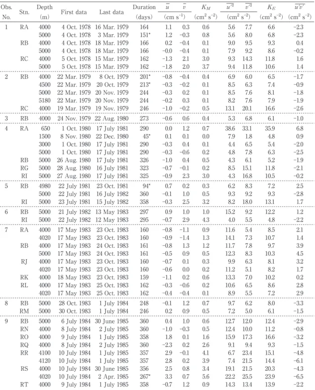
3. General statistics and combining records Table 2 shows the general statistics of all the
50 records obtained at 19 stations(Fig. 1). All calculations are done for the low-pass-filtered daily velocities. Statistics for Obs. 1 have already been reported(IMAWAKI, 1985). At abyssal depths(at 4000 m or deeper),the mean flow is weak and therefore, the kinetic energy per unit mass for the mean flow, or mean kinetic energy (KM)is small; it varies between 0.1 and 5.6 cm2 s-2. The kinetic energy per unit mass for meso-scale eddies, or eddy kinetic energy(KE)varies between 5 and 24 cm2s-2; it is an order of mag-nitude larger than the KM. This indicates that the site is located in the mid-ocean.
Time-space averages of those individual statis-tics at abyssal depths are calculated with weight of measurement duration and listed at the bot-tom of Table 2. The present 47 records at abys-Fig. 3 Time series of velocity and temperature observed at 4000 m depth at Stn. RA during Obs. 1. Panel(a)
is the raw data sampled at 30Ȃminute interval and(b)their low-pass-filtered data. From top to bottom in each panel, current speed(S; cm s-1),current direction(D; degrees, clockwise from the true
north),tem-perature(T; degrees Celsius),eastward velocity-component(U; cm s-1)and northward one(V; cm s-1)
sal depths provide the sum of 11, 660 day(32 year)data. Records obtained at several depths at the same station may not be independent from each other for the low-frequency fluctua-tions and therefore, incomplete records are ex-cluded first, if any, and then remaining complete records are weighted to represent one record at that station, except for Stn. RY, where the longer record is chosen. The data used for calculation of averages are totally 8830 day(24 year)data, and therefore, those statistics are considered to be representative values at the present site. The time-space average u and v components (-0.29 and 0. 71 cm s-1, respectively)are small. The average zonal and meridional variances(10 and 11 cm2 s-2, respectively)are almost equal to each other. The KE(11 cm2 s-2)is about 40 times larger than the KM(0. 3 cm2 s-2). Note that the KMlisted in the table is calculated from the average u and v components; the average of individual KMʼs is 1.5 cm2s-2.
For shallower flow field, three records were obtained at 650, 1500 and 3000 m depths at Stn. RA during Obs. 4. The record at 3000 m depth shows very similar features to those at 5000 m depth, in the time series of low-pass-filtered ve-locity and the general statistics. The record at 1500 m depth is too short to discuss mesoscale eddies but the hourly raw data shows an
inter-esting phenomenon of unusually long-lived iner-tial oscillation. The flow direction continues to change clockwise quite regularly for more than 40 days without any major disturbances or inter-ruption(not shown here). The average oscilla-tion period is estimated to be 22.8 h(41.8 days for 44 cycles),which is a little shorter than the local inertial period of 23. 93 h. The record at 650 m depth shows quite different features; zonal and meridional variances and KE are sev-eral times larger than those at 5000 m depth (Table 2).
At Stn. RB, moored current-meters were maintained continuously during all the nine ob-servations; each mooring was located within 10 km from the mean position. By combining those records, a long continuous record was obtained at 5000 m depth for 2462 days(6.7 years)from October 1978 through June 1985 as shown in Fig. 5. For Obs. 3, no current-meter was moored at 5000 m depth, and it is justifiably made up for by the record at 4000 m depth, because low-pass-filtered daily velocities at those abyssal depths at the same station are similar to each other as shown at beginnings of Sections 4 and 5. At Stn. RC, a continuous record was obtained at 4000 m depth for 411 days from October 1978 through November 1979; each mooring was located with-in 1 km from the mean position. At Stn. RI, a con-Fig. 4 Godin filter. Panel(a)shows the distribution of weights to be put
on 71 hourly data. Panel(b)shows the square of filter response factor as a function of fluctuation period.
Table 2. Statistics of lowȂpassȂfiltered daily velocities from 50 individual records. Symbol u(v)denotes east-ward(northward)velocityȂcomponent; overbar denotes temporal average over the record length and prime denotes deviation from it; KM(KE)denotes mean(eddy)kinetic energy. TimeȂspace
averages of those individual statistics at abyssal depths(see the text)are shown at the bottom.
Obs.
Stn. Depth First data Last data Duration KM
K E No. (m) (days) (cm sȂ1) (cm2sȂ2) (cm2sȂ2) (cm2sȂ2) (cm2sȂ2) 1 RA 4000 4 Oct. 1978 16 Mar. 1979 164 1.1 0.3 0.6 5.6 7.7 6.6 Ȃ2.3 5000 4 Oct. 1978 3 Mar. 1979 151* 1.2 Ȃ0.3 0.8 5.6 8.0 6.8 Ȃ2.3 RB 4000 4 Oct. 1978 18 Mar. 1979 166 0.2 Ȃ0.4 0.1 9.0 9.5 9.3 0.4 5000 4 Oct. 1978 18 Mar. 1979 166 Ȃ0.0 Ȃ0.4 0.1 7.9 9.2 8.6 Ȃ0.2 RC 4000 5 Oct. 1978 15 Mar. 1979 162 Ȃ1.3 2.1 3.0 9.3 14.3 11.8 1.6 5000 5 Oct. 1978 15 Mar. 1979 162 Ȃ1.8 2.0 3.7 9.4 11.8 10.6 1.4 2 RB 4000 22 Mar. 1979 8 Oct. 1979 201* Ȃ0.8 Ȃ0.4 0.4 6.9 6.0 6.5 Ȃ1.7 4500 22 Mar. 1979 20 Oct. 1979 213* Ȃ0.3 Ȃ0.2 0.1 8.5 6.3 7.4 Ȃ0.9 5000 22 Mar. 1979 20 Nov. 1979 244 Ȃ0.3 0.2 0.1 8.5 7.6 8.1 Ȃ1.8 5180 22 Mar. 1979 20 Nov. 1979 244 Ȃ0.2 0.3 0.1 8.2 7.6 7.9 Ȃ1.9 RC 4000 19 Mar. 1979 19 Nov. 1979 246 Ȃ1.0 Ȃ0.2 0.5 13.1 20.1 16.6 Ȃ2.6 3 RB 4000 24 Nov. 1979 22 Aug. 1980 273 Ȃ0.6 0.6 0.4 5.3 6.8 6.1 Ȃ1.0 4 RA 650 1 Oct. 1980 17 July 1981 290 0.0 1.2 0.7 38.6 33.1 35.9 6.8 1500 8 Nov. 1980 22 Dec. 1980 45* 0.1 0.1 0.0 7.9 1.8 4.8 0.9 3000 1 Oct. 1980 17 July 1981 290 Ȃ0.3 0.4 0.1 4.4 6.5 5.4 Ȃ2.0 5000 1 Oct. 1980 17 July 1981 290 Ȃ0.3 Ȃ0.6 0.2 4.8 7.8 6.3 Ȃ2.5 RB 5000 26 Aug. 1980 17 July 1981 326 Ȃ1.0 0.4 0.5 4.3 6.1 5.2 Ȃ1.9 RG 5000 28 Aug. 1980 16 July 1981 323 Ȃ0.7 Ȃ0.1 0.2 8.5 15.1 11.8 Ȃ2.1 RI 5000 27 Aug. 1980 17 July 1981 325 Ȃ0.9 2.3 3.0 4.3 16.8 10.5 Ȃ0.2 5 RB 4980 22 July 1981 23 Oct. 1981 94* 0.7 0.2 0.3 6.2 8.3 7.2 2.5 5000 22 July 1981 16 July 1982 360 Ȃ0.1 1.0 0.5 9.3 9.2 9.3 Ȃ2.8 RI 5000 23 July 1981 15 July 1982 358 Ȃ0.3 2.5 3.2 8.2 18.0 13.1 1.7 6 RB 5000 21 July 1982 13 May 1983 297 0.9 1.0 1.0 15.2 9.2 12.2 1.2 RI 5000 22 July 1982 12 May 1983 295 Ȃ0.7 2.9 4.3 4.0 5.5 4.8 Ȃ2.2 7 RA 4000 17 May 1983 23 Oct. 1983 160 Ȃ0.8 Ȃ1.1 0.9 11.6 5.4 8.5 2.1 4020 17 May 1983 23 Oct. 1983 160 Ȃ0.9 Ȃ1.4 1.3 14.1 7.3 10.7 1.4 RB 4000 17 May 1983 24 Oct. 1983 161 Ȃ0.8 1.3 1.2 11.7 7.8 9.7 3.9 5000 17 May 1983 24 Oct. 1983 161 Ȃ0.5 0.9 0.5 12.3 8.3 10.3 4.5 RJ 4000 17 May 1983 23 Oct. 1983 160 Ȃ0.7 0.1 0.3 9.9 6.3 8.1 3.2 4020 17 May 1983 23 Oct. 1983 160 Ȃ0.6 0.0 0.2 11.2 5.1 8.2 1.7 RK 4000 18 May 1983 23 Oct. 1983 159 Ȃ1.1 0.2 0.6 13.3 7.0 10.2 0.2 RL 4000 17 May 1983 25 Oct. 1983 162 Ȃ0.3 Ȃ0.6 0.2 10.6 6.5 8.6 2.8 4020 17 May 1983 25 Oct. 1983 162 Ȃ0.4 Ȃ0.4 0.1 8.9 5.5 7.2 2.9 8 RB 5000 28 Oct. 1983 1 July 1984 248 Ȃ0.1 1.2 0.7 9.7 6.2 8.0 Ȃ3.3 RM 5000 30 Oct. 1983 1 July 1984 246 0.2 0.9 0.5 7.2 5.0 6.1 Ȃ1.5 9 RB 5000 6 July 1984 30 June 1985 360 0.4 1.0 0.6 12.7 12.0 12.4 Ȃ2.9 RN 4000 8 July 1984 2 July 1985 360 Ȃ1.0 Ȃ0.3 0.5 12.4 10.0 11.2 Ȃ0.8 RO 4000 9 July 1984 1 July 1985 358 1.8 0.1 1.6 15.9 17.3 16.6 Ȃ3.2 RQ 4000 8 July 1984 2 July 1985 360 Ȃ2.3 0.2 2.6 9.1 9.4 9.3 Ȃ1.5 RR 4100 10 July 1984 1 July 1985 357 2.9 Ȃ0.1 4.1 6.7 23.4 15.1 Ȃ4.8 4120 10 July 1984 1 July 1985 357 2.8 0.2 3.9 7.4 21.5 14.4 Ȃ6.1 RS 4000 10 July 1984 30 June 1985 356 2.5 0.8 3.4 19.1 21.5 20.3 Ȃ4.3 4020 10 July 1984 2 Apr. 1985 267* 3.3 0.7 5.6 22.2 25.5 23.9 Ȃ6.5 RT 4000 9 July 1984 1 July 1985 358 Ȃ0.7 1.2 0.9 14.3 13.4 13.9 Ȃ2.2
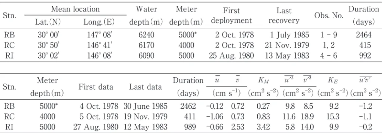
tinuous record was obtained at 5000 m depth for 989 days(2.7 years)from August 1980 through May 1983; each mooring was located within 2 km from the mean position. Table 3 shows the statis-tics of the three records. A part of the present time series of daily velocity has already been published(IMAWAKIand TAKANO, 1982; MIYAMOTO et al., 2017).
4. Mean flows
Differences of mean velocities between 4000 and 5000 m depths at the same station are small in five available comparison cases at Stns. RA, RB and RC(Table 2);standard deviations of dif-ferences of mean u and v components between the two depths are both 0.40 cm s-1, which is the same level as the estimated measurement er-ror(Section 2).That is to say mean velocities at
abyssal depths at the same station are similar to each other.
Figure 6 shows horizontal distribution of mean velocities at abyssal depths. A striking feature is the large anticyclonic vortex observed during Obs. 9 at 11 stations east of Stn. RB. This steady vortex, however, is beyond the scope of the pres-ent paper and described on a separate paper (IMAWAKI and TAKANO, 2019).The mean v com-ponent at Stn. RI(2. 5 cm s-1)is remarkably large. It comes from a stable mean flow toward north-northwest; means of v component during Obs. 4, 5 and 6 are 2.3, 2.5 and 2.9 cm s-1, respec-tively(Table 2).
At Stn. RB, nine observations were carried out continuously(Table 1 and Fig. 5).The mean ve-locity during each observation is shown in Fig. 7. Those mean velocities are weak and their
maxi-RU 4000 7 July 1984 1 July 1985 360 Ȃ2.0 0.6 2.2 10.4 10.6 10.5 Ȃ0.6 4020 7 July 1984 19 Oct. 1984 105* Ȃ2.8 1.5 5.1 14.3 3.3 8.8 0.9 RV 4020 7 July 1984 18 Nov. 1984 135* Ȃ3.0 0.7 4.7 11.4 2.2 6.8 Ȃ0.4 RX 4000 6 July 1984 7 June 1985 337* Ȃ0.3 1.4 1.0 14.9 13.0 14.0 Ȃ0.5 RY 4000 6 July 1984 7 June 1985 337* Ȃ1.4 0.9 1.4 12.0 9.1 10.5 Ȃ1.2 4020 6 July 1984 16 Mar. 1985 254* Ȃ1.3 0.8 1.1 11.9 11.2 11.6 Ȃ0.9 TimeȂspace average Ȃ0.29 0.71 0.29 10.19 11.37 10.79 Ȃ1.32
* Incomplete record which stopped before recovery due to battery trouble or instrumental failure
Table 3. Summary and statistics of long continuous records obtained by combining successive records. See Ta-ble 2 for notations.
Stn. Mean location Water Meter deploymentFirst recoveryLast Obs. No. Duration
Lat.(N) Long.(E) depth(m) depth(m) (days)
RB 30° 00' 147° 08' 6240 5000* 2 Oct. 1978 1 July 1985 1 Ȃ 9 2464
RC 30° 50' 146° 41' 6170 4000 2 Oct. 1978 21 Nov. 1979 1, 2 415
RI 30° 02' 146° 08' 6090 5000 25 Aug. 1980 13 May 1983 4 Ȃ 6 992
Stn. Meter First data Last data Duration KM
K E depth(m) (days) (cm sȂ1) (cm2sȂ2) (cm2sȂ2) (cm2sȂ2)(cm2sȂ2) RB 5000* 4 Oct. 1978 30 June 1985 2462 Ȃ0.12 0.72 0.27 9.8 8.5 9.2 Ȃ1.2 RC 4000 5 Oct. 1978 19 Nov. 1979 411 Ȃ1.06 0.73 0.83 11.6 18.9 15.3 Ȃ1.1 RI 5000 27 Aug. 1980 12 May 1983 989 Ȃ0.66 2.53 3.42 5.8 14.0 9.9 Ȃ0.2 * For Obs. 3, velocities at 4000 m depth are used instead of 5000 m(see the text).
mum speed is only 1. 4 cm s-1 during Obs. 6. Their v components are positive, except during Obs. 1. Their combined record shows followings (Table 3).The overall mean velocity during sev-en years is less than 1 cm s-1 in speed and di-rected to the north; the mean u(v)component is -0.12(0.72)cm s-1(Fig. 7).The K
M(0.3 cm2 s-2)is very small. Those statistics are quite similar to the time-space averages of all individu-al statistics at abyssindividu-al depths(Table 2).
Errors of those estimated mean u and v com-ponents due to low-frequency fluctuations are
evaluated at the 95 % confidence level, following ZENKand MÜLLER(1988)and TALLEYet al.(2011), as follows. The standard error Se is given by σ0/√Nd, where σ0 is the standard deviation of the original time series and Ndthe degrees of freedom. The degrees of freedom is given by Tr/ i, where Tris the record length and ithe integral timescale estimated approximately by integrating the autocorrelation function until its first zero-crossing. Assuming normal distribu-tion, the error ε of the estimated mean at the 95 % confidence level is given by tsSe, where ts,
Fig. 5 Time series of low-pass-filtered daily velocity obtained at 5000 m depth at Stn. RB from 4 October 1978 through 30 June 1985. For Obs. 3, velocities at 4000 m depth are used. Each stick represents a daily velocity vector(upward north). The abscissa is time in year-day. Arrowheads indicate exchange of moorings. Nu-merals indicate observation numbers.
the Studentʼs t-variable is about 2.0 when the de-grees of freedom is larger than 27. Those proper-ties for the present combined record at Stn. RB are shown in Table 4. The mean v component (0.72 ± 0. 35 cm s-1)is positive significantly, while the mean u component (-0.12 ± 0.44 cm s-1)is not significantly different from zero. Esti-mated means also include the measurement er-ror, which is not discussed here.
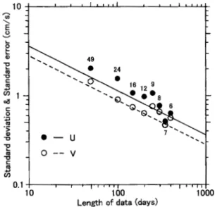
It is interesting to examine how a shorter-term “mean” fluctuates around a long-shorter-term mean, which is regarded to be closer to the true mean, and how it converges with increasing data
used, on real data. The present seven-year long data can provide many “means” estimated for shorter durations. For example, “means” for 200 days can be estimated in 12 independent cases; the “mean” u(v)components vary between -1.6 and 2.2 cm s-1(-0.4 and 1.7 cm s-1)with standard deviation of 1.0(0.6)cm s-1. Depend-ence of standard deviation of those “means” upon the length of data used for estimation is shown in Fig. 8. The figure also shows the standard er-ror Seas a function of record length. The stand-ard deviation decreases with increasing data length quite similarly to the standard error, al-Fig. 6 Horizontal distribution of mean velocities at abyssal depths during individual
observa-tions(thin arrows; Table 2)and those from three combined records(thick arrows; Table 3). Velocities at 4000 m depth are shown, except 5000 m depth velocities at Stns. RB, RG and RI, and for Obs. 4 at Stn. RA. Three arrows at Stn. RA are for Obs. 1, 4 and 7. At Stn. RB, the mean velocity during Obs. 9 is shown as well as that from the combined record. Selected sta-tion names are shown with the first “R” omitted. Darker gray indicates shallower depth, with contours of 500 m interval.
though the standard deviation is 1.2(1.1)times larger than the standard error for the u(v) component, on an average, in the present case. 5. Statistics of mesoscale eddies
In some observations, records at both 4000 and 5000 m depths are available at the same sta-tion. Their low-pass-filtered daily velocities are very similar to each other and no significant
dif-ferences are recognized in their time series(not shown here);their statistics are basically similar to each other(Table 2).It suggests that the ve-locity field of mesoscale eddies is almost uniform vertically at abyssal depths.
Figure 9 shows KEʼs during individual
obser-Fig. 7 Mean velocities for nine individual observa-tions at 5000 m depth at Stn. RB. Numerals indi-cate observation numbers. Also shown is the mean velocity(M)from the long combined re-cord(Fig. 5),with its estimated error at the 95 % confidence level(broken line).
Table 4. Estimating errors of mean u and v components for almost seven years at 5000 m depth at Stn. RB.
u v
Standard deviation σ0(cm s-1) 3.1 2.9
Record length Tr(days) 2462 2462
Integral timescale i(days) 12.3 8.7
Degrees of freedom Nd 200 283
Standard error Se(cm s-1) 0.22 0.17
Error on 95 % confidence level (cm s-1) 0.44 0.35
Mean (cm s-1) Ȃ0.12 ± 0.44 0.72 ± 0.35
Fig. 8 Dependence of standard deviation of “means” upon the length of data used for their es-timations. Each numeral is the number of “means” estimated for a certain data length. Two lines show the standard error Se[=σ0√( i/Tr)
with σ0 and i in Table 4] as a function of
re-cord length(Tr).Dots and the solid line are for u
component, and open circles and the broken line are for v component. The figure is drawn by uti-lizing the seven-year long record at Stn. RB.
vations at Stn. RB(Fig. 5).Fluctuation of the KE is large; the maximum KE(12.4 cm2s-2)is more than two times larger than the minimum KE(5.2 cm2s-2).The figure also shows the partition of zonal and meridional KEʼs. Ratios of meridional to zonal KEʼs vary between 0.6 and 1.4, with a mean of 0.9. The long combined record at Stn. RB(Fig. 5 and Table 3)shows followings. The flow direction of daily velocity changes mostly counterclockwise. The zonal variance(10 cm2 s-2)is similar to the meridional variance(9 cm2 s-2). The K
E(9. 2 cm2 s-2)is more than 30 times larger than the KM(0.3 cm2 s-2).Those statistics are quite similar to the time-space averages of all individual statistics at abyssal depths(Table 2).
For the combined record at Stn. RC(Table 3), the meridional variance(19 cm2 s-2)is large, which results in large KE(15 cm2 s-2).Those two are also large for individual records(Obs. 1 and 2)compared with other stations(Table 2). For the combined record at Stn. RI, the meri-dional variance(14 cm2 s-2)is more than two
times larger than the zonal variance(6 cm2s-2). At Stn. RR, both two records(separated by 20 m in vertical)show that the meridional variance(22 cm2 s-2)is three times larger than the zonal variance(7 cm2 s-2), which is unique in the present statistics. At Stn. RS, both two records (separated by 20 m in vertical)show large KEʼs (20 and 24 cm2 s-2),which are about twice of
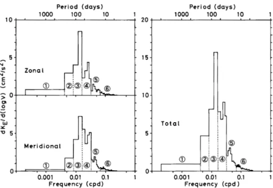
the overall time-space average(Table 2). 6. Frequency spectra
The seven-year long velocity record at 5000 m depth at Stn. RB(Fig. 5)gives statistically sig-nificant estimates of frequency spectra for the eddy kinetic energy(Fig. 10). Zonal and meri-dional power spectral densities are estimated from energy densities obtained by the fast Fouri-er transform method and avFouri-eraged ovFouri-er 10 fre-quencies. Hence spectra for the zonal and meri-dional KEʼ s are regarded as containing 20 de-grees of freedom, and their 95 % confidence limits are from 0.58 to 2.1 times individual esti-mates. The spectrum for the total KEis estimat-ed as the sum of those two and therefore, its con-fidence limits are somewhat narrower than that range.
For convenience, each spectrum is divided in-to six frequency bands. They are labeled “annu-al/secular scale,” “mesoscale I,” “mesoscale II,” “mesoscale III,” “monthly scale” and “rest.” Their period ranges and KEʼs contained in those bands are shown in Table 5, which also shows ratios of the meridional to zonal KEʼs.
Most of the total KE(78 %)is contained in the mesoscale I, II and III bands(period range of 31Ȃ235 days). Therefore, the three bands as a whole could be called an energy-containing or eddy-containing band(MODE GROUP, 1978). In the whole eddy-containing band, the zonal and meridional KEʼs are equal to each other(both, 3.5 cm2s-2).In the mesoscale I, the zonal K
Eis
Fig. 9 Eddy kinetic energies during nine individual observations at 5000 m depth at Stn. RB. Numer-als indicate observation numbers. Partition of zo-nal KE(shaded box)and meridional KE(blank
Fig. 10 Frequency spectra of eddy kinetic energy estimated from the seven-year long record at 5000 m depth at Stn. RB(Fig. 5).They are plotted in a variance-preserving form, i.e., an area below the curve represents energy contents in the corresponding frequency range. Symbol ν denotes frequency in cycle per day. Spectra of zonal, meridional and total KEʼs are
shown. Each spectrum is divided into six frequency bands, whose ranges are shown by dot-ted lines and whose reference numbers are indicadot-ted by circled numerals. See Table 5 for de-tails.
Table 5. Zonal, meridional and total eddy kinetic energies contained in six frequency bands of the spectra shown in Fig. 10. Also shown are labels of frequency bands, their period ranges, and ratios of meridional to zonal KEʼs. Small
discrep-ancy among numerals is due to rounding lower digits.
Label of Period range Zonal KE Meridional KE Total KE Ratio
frequency band (days) (cm2s-2)
1 Annual/secular scale 235 Ȃ 4924 1.0 0.2 1.2 0.2 2 Mesoscale I 120 Ȃ 235 0.9 0.5 1.4 0.6 3 Mesoscale II 61 Ȃ 120 1.7 1.6 3.4 0.9 4 Mesoscale III 31 Ȃ 61 0.9 1.4 2.3 1.6 5 Monthly scale 16 Ȃ 31 0.3 0.3 0.6 1.3 6 Rest 2 Ȃ 16 0.1 0.1 0.2 1.2 Whole 2 Ȃ 4924 4.9 4.2 9.2 0.9
dominant, while in the mesoscale III, the meri-dional KEis dominant. In the mesoscale II, they are almost equal to each other. In the annual/
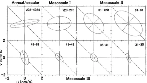
secular scale, the zonal KE is more than four times larger than the meridional KE. In the monthly scale, they are almost equal to each oth-Fig. 11 Current ellipses of lowest eight frequency bands of spectra shown in oth-Fig. 10.
Numerals at upper-right corner of each panel show the period range(in days)of that frequency band. Solid lines are u and v axes, dashed lines are major and minor axes, and dotted lines indicate the northwest/southeast direction.
Fig. 12 Conceptual figures of dispersion relation of barotropic Rossby waves (circles)for three periods and selected wavenumber vectors(arrows).Panel (a)is for the period of 180 days and a wavenumber vector directed to the north-northwest with a wavelength of 290 km,(b)for 90 days and the south-west, with 360 km, and(c)for 45 days and the west-southsouth-west, with 570 km. Symbol k(l)denotes the zonal(meridional)wavenumber.
er. In the rest, they are trivially small.
Those spectral features are shown in a differ-ent way as currdiffer-ent ellipses based on rotary spec-trum analysis(Fig. 11). In the annual/secular scale and mesoscale I, the major axis is almost parallel to the u-axis, and zonal fluctuations are dominant. In the mesoscale II(two panels),the major axis is parallel to the northwest/southeast, and zonal and meridional fluctuations are compa-rable. In the mesoscale III(four lower panels), the major axis is parallel to the north-north-west/south-southeast, and meridional fluctua-tions are dominant.
Both zonal dominance in the longer-period bands and meridional dominance in the shorter-period band are understood qualitatively by dif-ference in phase propagation direction of fluctua-tions, if the fluctuations are assumed as plane barotropic Rossby waves having moderate wavelengths of hundreds of kilometers, as point-ed out by IMAWAKIand TAKANO(1982).The as-sumption of plane waves is supported by MIYAMOTOet al.(2019).Figure 12 shows this sit-uation conceptually. The plane Rossby wave of a longer period(Panel a; mesoscale I)is able to have a wavenumber vector(with a moderate magnitude)directed nearly to the north or south; its associated motion is dominantly zonal. On the other hand, the Rossby wave of a shorter period (Panel c; mesoscale III)is able to have a moder-ate wavenumber vector directed nearly to the west; its associated motion is dominantly meri-dional. The Rossby wave of a moderate period (Panel b; mesoscale II)is able to have a moder-ate wavenumber vector directed to the south-west or northsouth-west; its associated motion is of no dominance. The wavelengths shown in Fig. 12 are similar to those estimated by fitting a set of barotropic Rossby waves to fluctuations at sev-eral stations in the present site(IMAWAKI, 1985).
7. Vorticity balance
Theoretically, the motion of mid-ocean meso-scale eddies is described as follows. Let x(y)be the eastward(northward)coordinate, and(u, v) the corresponding velocity components. The Rossby number Ro is defined as U/fL, where U is a characteristic horizontal velocity scale, f the Coriolis parameter and L a characteristic hori-zontal length scale. Taking U = 10 cm s-1, f = 10-4s-1and L = 100 km, the R
ois 0.01, which is small enough for equations to be developed in an asymptotic series in Ro, providing the quasi-geostrophic regime(PEDLOSKY, 1996)as follows.
Under the Boussinesq approximation and hy-drostatic approximation, the quasi-geostrophic field is described as follows. The horizontal ve-locity v is expanded as v = v0+ v1+…, where v0=(u0, v0)is the lowest order velocity and v1 the first order velocity, being as small as Ro v0. The lowest order velocity v0 is in geostrophic balance and horizontally non-divergent.
f0ku× v0= - -1 p (1)
・ v0= 0. (2)
Here kuis the upward unit-vector perpendicular to the x-y plane, f0the Coriolis parameter at the origin, the water density and p the pressure, of the lowest order. The equation for the vertical component of relative vorticity =[v0x- u0y]of the lowest order is
t+ v0・ + v0+ f0 ・ v1= 0. (3) Here notation tmeans time derivative of a scal-er propscal-erty , and x( y)means x(y)deriva-tive of . The parameter is the meridional gra-dient of Coriolis parameter at the origin; is 0.20 × 10⁻¹²cm-1s-1at 30°N. Equation(3)shows that the local time change of relative vorticity is
balanced with the sum of the horizontal advec-tion of relative vorticity, horizontal advecadvec-tion of planetary vorticity(beta-effect)and divergence of the first order horizontal velocity(vertical stretching).If the flow is associated with baro-tropic planetary Rossby waves, the vorticity equation becomes the linear non-divergent vor-ticity balance, which is simply
t+ v0= 0. (4)
On the basis of this theoretical framework, we examine how well the local change of relative vorticity is balanced with the advection of plane-tary vorticity[Eq.(4)]for actual mesoscale eddies, using the present current-meter data. Observed horizontal velocity Vobs represents mostly the lowest order velocity v0because the first order velocity v1 is too small to be distin-guished from measurement error. The
diver-gence of observed horizontal velocity ・ Vobs estimated by finite difference includes an error due to smaller-scale fluctuations which cannot be resolved by the present observations, as well as the measurement error. It means that the calcu-lated divergence may not be zero, although the divergence should be zero theoretically[Eq.(2)]. Therefore, the value of calculated divergence can be regarded as an error in both measure-ment and finite differencing(IMAWAKI, 1983).
・ Vobs= Error. (5)
The first three terms in Eq.(3)can be estimat-ed from observestimat-ed velocities, but the last term (vertical stretching)cannot be estimated
direct-ly.
To examine the vorticity balance, field meas-urements were carried out twice. The first was a set of five stations in a cross pattern centered at Fig. 13 Sequence of 10Ȃday interval snapshots of 10Ȃday mean velocities at 4000 m
depth during Array-83. The year-day of 1983 is shown at the upper-left corner of each panel. On underlined days, vorticity balance is examined.
Stn. RJ with zonal and meridional separations of 24 km(Fig. 1). It was carried out from May through October 1983 as Array-83(Obs. 7).The second was a set of 13 stations in a diamond shape centered at Stn. RT with separations of 25 km. It was carried out from July 1984 through July 1985 as Array-84(Obs. 9).
7.1 Array-83
Figure 13 shows a sequence of 10Ȃday mean velocities at 4000 m depth during Array-83. Ed-dies having a speed of 10 cm s-1 travel in the site. Figure 14 shows variables concerning the vorticity balance at Stn. RJ, at 20Ȃday interval. Estimated variables are temporally independent from each other because the time interval is much longer than integral timescales of u and v components(Table 4).In this section, all varia-bles are based on 20Ȃday mean velocities; target-ed target-eddies are having temporal scales of more
than several-ten days(periods longer than the mesoscale III). Horizontal derivatives are esti-mated by finite difference of velocities with a spatial interval of 48 km, in a straightforward manner. Their error is estimated to be 0.09 × 10⁻⁶s-1from the error(0.3 cm s-1)of u and v components. The station-spacing is fine enough compared with the typical horizontal scale of fluctuations, which is inferred from the lag (70Ȃ90 km)of first zero-crossing of transverse
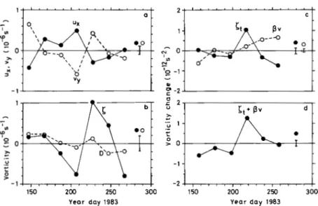
correlation function of velocity fluctuations. After subtracting averages during the array observation, horizontal derivatives u0x and v0y are estimated[Fig. 14(a)].They have general-ly opposite signs and almost equal magnitudes; their correlation coefficient (-0.89) is very high in magnitude, and standard deviations of u0xand v0y are almost the same, suggesting that they are balanced well with each other. Horizontal di-vergence calculated from the two is shown in Fig. 14 Time series of various properties concerning the vorticity balance at
Stn. RJ during Array-83. Panel(a)is for u0x(dots)and v0y(open circles),
(b)for (dots)and calculated horizontal divergence(D ; open circles),(c) for t(dots)and v0(open circles),and(d)for the sum of these two( t+
v0).In each panel, vertical bars on the right-hand side indicate
Fig. 14(b).As shown in Eq.(5),the calculated divergence is regarded as an error; i.e., its stand-ard deviation(0.18 × 10⁻⁶s-1)gives the error in addition or subtraction of two similar horizon-tal derivatives. Figure 14(b)also shows the es-timated relative vorticity . Its standard devia-tion(0.61 × 10⁻⁶s-1)is more than three times larger than the estimated error.
The local change of relative vorticity tis esti-mated from difference of ʼs separated by 20 days. The advection of planetary vorticity v0is estimated from the v component at Stn. RJ. Those two are shown in Fig. 14(c).The stand-ard deviation of v0(0.43 × 10⁻¹² s-2)is not much different from that of (0.54 × 10t -12s-2),
but their correlation coefficient (-0.27) is rather low. Figure 14(d)shows the sum of these two, which is the departure from the linear non-divergent vorticity balance[Eq.(4)].The sum is small in half of six cases(for year-days 178, 238 and 258),being below or close to its estimat-ed error(0.15 × 10⁻¹²s-2),but large in other cases, especially on year-day 218, for which a large increase of from year-days 208 to 228 can-not be accounted for by v0. The horizontal ad-vection of relative vorticity cannot be estimated from the Array-83 data.
As conclusion of this subsection, the local change of relative vorticity is balanced basically with the advection of planetary vorticity but oc-Fig. 15 Same as oc-Fig. 13, but for Array-84 and serial year-day of 1984. At Stns. RB and RR, velocities at 5000
casionally some unknown terms are required to complete the vorticity balance.
7.2 Array-84
Figure 15 shows a sequence of 10Ȃday mean velocities at 4000 m depth during Array-84. The flow is very smooth horizontally and organized well; for example, velocity vectors are like a school of swimming-fish on year-days 242, 372 and 432, and well-organized anticyclonic eddies are seen on year-days 252 and 402. The flow is dominated by anticyclonic patterns. It is because the flow is heavily biased by the steady vortex (Fig. 6)having strong negative vorticity of -1.1 × 10⁻⁶ s-1 at Stn. RT and RP(IMAWAKI and TAKANO, 2019).Time series of daily velocities at all stations show that the flow direction changes mostly counterclockwise(not shown here).
In the following analysis, missing data at Stn. RP(RW)are filled by averaging data from Stns. RO, RN, RQ and RT(RR and RB). At Stn. RV, data are available only during first 135 days, and so we are forced to use data extrapolated linear-ly from Stns. RT and RU for the remaining peri-od. At Stns. RX and RY, the usable data stopped before the end of array observation, and so the analysis on vorticity balance is stopped at that time(year-day 525).
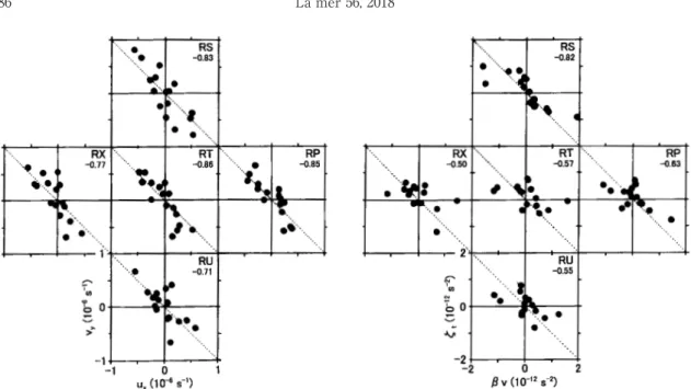
After subtracting averages during the array observation, analysis similar to Array-83 is car-ried out for Stns. RS, RP, RT, RX and RU, using data at five nearby stations separated by 25 km. The results are shown as scatter plots(Figs. 16 and 17).Horizontal derivatives u0xand v0yhave generally opposite signs and almost equal magni-tudes(Fig. 16).Their correlation coefficients are very high in magnitude at all five stations. For the overall average of 80 cases, the correlation coefficient is -0.80, and standard deviations of u0xand v0y are similar to each other, suggesting
Fig. 16 Scatter plots of u0x versus v0y at five
sta-tions, whose names are shown at the upper-right corner of each panel, during Array-84. Numerals below station names are correlation coefficients of 16 cases each. Dotted lines indicate the perfect out-of-phase correlation.
Fig. 17 Same as Fig. 16, but for plots of v0 versus t, and 15 cases.
that the two variables are balanced very well. Vorticity balances between the local change of relative vorticity t and advection of planetary vorticity v0 at the five stations are shown in Fig. 17. The two properties have generally oppo-site signs and almost equal magnitudes. Their correlation coefficients are high at Stn. RS. They are not so high at other stations but significantly different from zero at the 95 % confidence level. The overall correlation coefficient of 75 cases is -0.61, which is high enough in magnitude to be significantly different from zero at the 95 % con-fidence level. The overall standard deviation of t is 0. 65 × 10-12 s-2and that of v
0 is 0. 45 × 10-12s-2.
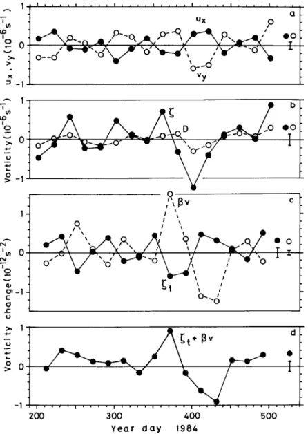
The same results as the scatter plot for Stn. RT in Fig. 16 are shown as time series of u0xand v0yin Fig. 18(a).They have generally opposite
signs and similar magnitudes; their correlation coefficient (-0.86) is very high in magnitude and standard deviations of u0xand v0yare simi-lar to each other, suggesting well-balanced varia-tions. The time series of sum of the two, namely the calculated horizontal divergence is shown in Fig. 18(b);its standard deviation(0.18 × 10⁻⁶ s-1)gives the error of the relative vorticity and is numerically the same as the correspond-ing one in Array-83. The standard deviation of (0. 69 × 10-6 s-1)is almost four times larger
than the error.
Similarly, the same results as the scatter plot for Stn. RT in Fig. 17 are shown as time series of tand v0in Fig. 19(a).Their correlation coeffi-cient (-0.57) is significantly different from zero at the 95 % confidence level as mentioned above. The standard deviation of v0(0.64 × 10⁻¹²s-2)
Fig. 18 Time series of properties concerning the vorticity balance at Stn. RT during Array-84. Panel(a)is for u0x(dots)and v0y(open circles),and
(b)for (dots)and calculated horizontal divergence(D ; open circles).In each panel, a vertical bar on the right-hand side indicates corresponding estimated error.
is larger than that of t(0.38 × 10⁻¹²s-2).The sum of these two[Fig. 19(b)]is small in about half of 15 cases(for year-days 212, 252, 292, 332, 392, 472 and 492),being below or close to its
esti-mated error(0. 15 × 10-12 s-2), but large on year-days 232, 372, 412, 432 and 452. Especially on year-days 372, 412 and 432, the t is over-balanced by the large v0.
Fig. 19 Time series of various terms of vorticity balance at Stn. RT during Array-84. Panel(a)is for t(dots)and v0(open circles),(b)for the sum
of these two( t+ v0; dots)and advection of relative vorticity(v0・ ;
open circles),and(c)for the sum of those three( t+ v0+ v0・ ).In
each panel, vertical bars on the right-hand side indicate corresponding es-timated errors.
Figure 19(b)also shows the horizontal ad-vection of relative vorticity v0・ , estimated from the velocity at Stn. RT and gradient of over Stns. RS, RP, RU and RX. The advection of
accounts for the above sum( t+ v0)to some extent in several cases(for year-days 312, 332, 352, 372, 392 and 452),but does not account for
in other cases, having large negatives(for year-days 232, 412 and 432).In short, the horizontal advection of relative vorticity accounts for the imbalance between the local change of relative vorticity and advection of planetary vorticity in some cases, but makes the imbalance worse in other cases.
Fig. 20 Same as Fig. 14, but for Stn. RT during Array-84, using data at Stns. RR, RN, RV, RB and RT to examine a larger-scale balance.
Finally, the vorticity balance is examined on a larger scale, using data at five stations separated by 50 km, namely Stns. RR, RN, RV, RB and RT. Time series of u0xand v0yat Stn. RT are shown in Fig. 20(a). They have generally opposite signs and almost equal magnitudes; their correla-tion coefficient (-0.92) is very high in magni-tude and standard deviations of u0xand v0y are almost the same. Figure 20(b)shows the hori-zontal divergence calculated from the two and ; the standard deviation of (0.50 × 10⁻⁶s-1)is much larger than that of horizontal divergence (0.15 × 10⁻⁶ s-1), which gives the error of . The v0(the same as the smaller scale)and t are shown in Fig. 20(c).Their correlation coef-ficient (-0.80) is much higher in magnitude than the smaller scale. The standard deviation of v0is larger than that of t(0.37 × 10⁻¹²s-2). The sum of these two [Fig. 20(d)] is small in about half of 15 cases but large on year-days 372, 412 and 432, where t is again over-balanced by the large v0. The relation between the two is a little better on the larger scale than smaller scale.
As conclusion of this subsection, the local change of relative vorticity is balanced basically with the advection of planetary vorticity on both smaller and larger scales. In some cases, the hori-zontal advection of relative vorticity accounts for the imbalance between the two, but makes it worse in other cases; the vorticity balance of mesoscale eddies has not yet been completed. 8. Discussions
Records at 5000 m depth at Stn. RI show a sta-ble north-northwestward flow. The station is lo-cated at 40 km east of Stn. TA(30°00'N, 145° 45'E),where a strong south-southeastward mean flow along local isobaths was observed during 1978Ȃ1982, with bottomward intensification, namely the speed increase from 3.2 cm s-1 at
4000 m depth to 7.2 cm s-1at 5800 m depth(50 m above the bottom)(Keisuke Taira, personal communication; Miyamoto et al., 2019).The sta-ble flow at Stn. RI might be a part of the local circulation associated with this strong flow at Stn. TA.
Records at 4100 m depth level at Stn. RR show unique dominance of the meridional variance over zonal variance. As shown in Fig. 1, the sta-tion is located at the foot of western slope of the seamount, which rises from 6300 m deep bottom up to 5400 m depth. The meridional dominance is probably due to preference of fluctuating flows along local isobaths, although a remarkable mean flow associated with the steady vortex is directed to the seamount(Fig. 6). This local dominance of meridional variance could disturb the examination of vorticity balance but the pos-sible distortion is not apparent in the Array-84 analysis.
A long velocity record for almost seven years was obtained at 5000 m depth at Stn. RB. This is probably one of the longest continuous records from moored current-meters at depth in the mid-ocean over the world, together with a similar long record at 1000 m depth in the eastern North Atlantic, where moorings were maintained dur-ing 1980Ȃ1986(ZENK and MÜLLER, 1988). The mean v component(0. 72 cm s-1)at 5000 m depth at Stn. RB is almost exactly equal to that of time-space average(0.71 cm s-1)of statistics of all records at abyssal depths in the present site, the mean u component of the former (-0.12 cm s-1)is close to that of the latter (-0.29 cm s-1),and the K
Eof the former(9.2 cm2s-2)is similar to that of the latter(10.8 cm2 s-2 ),sug-gesting that the record at Stn. RB represents the flow field at the present site quite well. On the other hand, the mean velocity at Stn. RB might be under the effect of the local steady vortex (Fig. 6; IMAWAKIand TAKANO, 2019).Therefore, it
is hard to definitely judge its representativeness of the site.
The eddy kinetic energy is compared with other locations. The level of KE at the present site(11 cm2 s-2)is comparable with that(12 cm2 s-2)at 4000 m depth at similar latitudes along 152°E(SCHMITZ, 1984).The present level is higher than that in the central North Pacific (TAFT et al., 1981)but lower than that in the Kuroshio Extension(SCHMITZ, 1984).It is compa-rable with the level of KE at abyssal depths in the MODE area(Schmitz, 1978).At Stn. RC, the KEis large, which might be due to the fact that the station is relatively near to the Kuroshio Ex-tension, considering that the KEat 4000 m depth along 152°E has the maximum(45 cm2s-2)at 35°N, namely the vicinity of the upper layer ex-pression of the Kuroshio Extension(SCHMITZ, 1984).
The spectral features of mesoscale eddies ob-tained in this study are compared with those of the three-year long first-half of the present re-cord(IMAWAKIand TAKANO, 1982).All the major features of the first-half spectra are found in the present spectra, with a finer resolution and in a wider frequency range. The spectral analysis shows zonal dominance of eddy motions in longer-period bands and meridional dominance in the shorter-period band. If the fluctuations are associated with barotropic Rossby waves, the dominance is understood in the vorticity balance [Eq.(4)]as follows. If the period of waves is longer(shorter), the local change of relative vorticity tis smaller(larger)and therefore, the advection of planetary vorticity v0 is smaller (larger), which means the meridional compo-nent v0is smaller(larger),i.e., the zonal(meri-dional)fluctuations are dominant. Those spec-tral features are also seen in spectra at 4000 m depth in the western North Atlantic(RICHMANet al., 1977), although zonal dominance of energy
in the annual scale is not definite. The zonal dominance of eddy fields in longer periods has been suggested by theoretical works(e.g., RHINES, 1977).On the other hand, the meridional eddy ki-netic energy is dominant in the temporal meso-scale band and even in the annual band at 1000 m depth in the eastern North Atlantic(ZENKand MÜLLER, 1988).
Concerning the vorticity balance, the local change of relative vorticity is balanced primarily with the advection of planetary vorticity, al-though the advection of relative vorticity and higher-order divergence may play some role in the balance. It is consistent with the earlier re-sults(IMAWAKI, 1983)obtained by using 10Ȃday mean velocities at 5000 m depth at five stations in the present site, whose station-spacing is somewhat similar to the present larger scale ex-amination.
The present study shows that mesoscale ed-dies at abyssal depths in mid-ocean are under-stood basically as fluctuations associated with plane barotropic Rossby waves. Recent studies show that mesoscale fluctuations at the present site having specific spectral peaks are explained by topographic Rossby waves better than plane-tary Rossby waves(MIYAMOTOet al., 2017; 2019); the former are influenced by the topographic beta-effect as well as planetary beta-effect. In the present analyses, topographic Rossby waves are indistinguishable from barotropic planetary Rossby waves. It is because wavelengths cannot be estimated from single-station data and there-fore, the dispersion relation of Rossby waves cannot be used for comparison. It is also because the higher-order divergence in the vorticity bal-ance, where the effect of bottom topography ap-pears as well as the baroclinicity, does not seem to be estimated reliably as the residual of first three terms of Eq.(3).
Array-84, missing data at three stations are made up for by linearly interpolated or extrapo-lated data. Scatter plots of u0x versus v0y and v0 versus t at five stations using those data (Figs. 16 and 17)do not show any difference among stations. Therefore, the interpolation and extrapolation seem to have worked well. Objec-tive analysis may improve filling the missing da-ta as well as spatial smoothing.
9. Summary
Velocities at abyssal depths were measured by moored current-meters in mid-ocean of the western North Pacific during 1978Ȃ1985. Cur-rent-meters were moored mostly at 4000 and 5000 m depths at various locations for several months to one year repeatedly, providing 50 ve-locity records. In the raw data, inertial oscilla-tions are apparent as well as diurnal and semi-diurnal tidal fluctuations. Those high-frequency fluctuations are filtered out numerically and low-pass-filtered daily velocities are used for the present analyses.
Time-space averages of statistics of 47 individ-ual records at abyssal depths show followings. The average zonal and meridional velocity-components are less than 1 cm s-1in magnitude. The average zonal and meridional variances are almost equal to each other. The eddy kinetic en-ergy is about 40 times larger than the mean ki-netic energy. Those statistics confirm that the site is located in typical mid-ocean apart from in-tense current zones. Both mean velocities and fluctuating velocities at abyssal depths at the same station are similar to each other.
A long velocity record for almost seven years was obtained at 5000 m depth at Stn. RB. This is probably one of the longest continuous records from moored current-meters at depth in the mid-ocean over the world. The overall mean velocity is directed to the north with a speed of less than
1 cm s-1. The mean meridional velocity-compo-nent is positive significantly at the 95 % confi-dence level, while the mean zonal component is not significantly different from zero. The zonal variance is similar to the meridional variance. The eddy kinetic energy is more than 30 times larger than the mean kinetic energy. Those sta-tistics are quite similar to the time-space averag-es of all individual statistics at abyssal depths mentioned above, suggesting that the long re-cord at Stn. RB represents the flow field at the present site quite well, although the mean veloci-ty might be under the effect of the local steady vortex.
This long velocity record at Stn. RB gives stat-istically significant estimates of frequency spec-tra for the eddy kinetic energy. Most of the eddy kinetic energy is contained in mesoscale bands I, II and III(period-rage of 31Ȃ235 days). In the three bands as a whole, zonal and meridional en-ergies are almost equal to each other. In the mes-oscale I(120Ȃ235 days)the zonal energy is dom-inant, while in the mesoscale III(31Ȃ61 days)the meridional energy is dominant. In the annual/ secular scale(295Ȃ4924 days)the zonal energy is highly dominant. Both zonal dominance in longer-period bands and meridional dominance in the shorter-period band are understood quali-tatively by difference in phase propagation di-rection of fluctuations, if the fluctuations are as-sumed as plane barotropic Rossby waves having wavelengths of hundreds of kilometers.
The vorticity balance of mesoscale eddies is examined by using those current-meter data. Relative vorticity is estimated from horizontal derivatives of 20Ȃday mean velocities. Its local change during 20 days is compared with the ad-vection of planetary vorticity, at five stations, providing 75 independent comparison cases. The overall correlation coefficient between the two properties of those cases is -0.61, which is high
enough to be significantly different from zero at the 95 % confidence level. The overall standard deviations of the two are not much different from each other. Therefore, the local change of relative vorticity is balanced primarily with the advection of planetary vorticity, although the ad-vection of relative vorticity and higher-order horizontal divergence may play some role in the balance.
Those results suggest that mid-ocean meso-scale eddies at abyssal depths are understood as primarily plane barotropic Rossby waves with possible modification.
Acknowledgements
We thank Mr. Masatoshi Miyamoto of the Uni-versity of Tokyo for informing the ETOPO1 bot-tom topography. We are grateful to two anony-mous reviewers and Prof. Masahisa Kubota of Tokai University for careful and critical reading of the manuscript and valuable comments. We also thank Mr. Keith Bradley of the Woods Hole Oceanographic Institution(at that time)for in-troducing SI to the mooring technique. [Affilia-tion is hereafter understood “at that time.”]The mooring observations were carried out under the lead of KT of the Institute of Physical and Chemical Research and later of the University of Tsukuba with collaboration of SI of Kyoto versity. We thank Mr. Satoshi Murata of the Uni-versity of Tsukuba for his helpful assistance. Mooring deployment and recovery were carried out on board the research vessel Hakuho Maru of the University of Tokyo, the research and training vessels Tokaidaigaku Maru II and Bosei Maru II of Tokai University(Table 1).We thank Captains and crews of those vessels for their ear-nest cooperation. The current measurements were done as a pre-operational survey for the disposal of low-level radioactive wastes, financial-ly supported by the Science and Technology
Agency through the Radioactive Waste Manage-ment Center. The data were processed at the Data Processing Center of Kyoto University. The work was partly supported by Grants-in-Aid from the Ministry of Education, Science and Culture. The present low-pass-filtered velocities are available at the Website of Japan Oceano-graphic Data Center; http: //www. jodc. go. jp/ jodcweb/JDOSS/.
References
AMANTE, C. and B. W. EAKINS(2009):ETOPO1 1 Arc-Minute Global Relief Model: Procedures, Data Sources and Analysis. NOAA Technical Memo-randum NESDIS NGDC-24. National Geophysical Data Center, NOAA. doi: 10.7289/V5C8276M. CREASE, J.(1962):Velocity measurements in the deep
water of the western North Atlantic, summary. J. Geophys. Res., 67, 3173Ȃ3176.
FU, L.-L. and R. MORROW(2013):Remote sensing of the global ocean circulation. In Ocean Circula-tion and Climate: A 21st Century Perspective. G. SIEDLER, S. M. GRIFFIES, J. GOULDand J. A. CHURCH (eds.),Academic Press, London, pp. 83Ȃ111. GODIN, G.(1972): The Analysis of Tides. Liverpool
University Press, 264 pp.
GREENE, A. D., D. R. WATTS, G. G. SUTYRIN and H. SASAKI(2012):Evidence of vertical coupling be-tween the Kuroshio Extension and topographi-cally controlled deep eddies. J. Mar. Res., 70, 719Ȃ747, doi: 10.1357/002224012806290723. HEINMILER, R. H.(1976):Mooring Operations
Techni-ques of the Buoy Project at the Woods Hole Oce-anographic Institution, W. H. O. I. Technical Re-port 76Ȃ69. Woods Hole Oceanographic Institu-tion, Woods Hole, Massachusetts, 94 pp.
IMAWAKI, S.(1983): Vorticity balance for mid-ocean mesoscale eddies at an abyssal depth. Nature, 303, 606Ȃ607, doi: 10.1038/303606a0.
IMAWAKI, S.(1985):Features of mesoscale eddies in the deep mid-ocean of the western North Pacific. Deep-Sea Res., 32, 599Ȃ611, doi: 10. 1016/0198Ȃ 0149(85)90046Ȃ9.
eddy kinetic energy spectrum in the deep west-ern North Pacific. Science, 216, 1407Ȃ1408, doi: 10.1126/science.216.4553.1407.
IMAWAKI, S. and K. TAKANO(2019):Steady vortex ob-served by moored current-meters at 4000 m depth in the western North Pacific.(to be pub-lished)
KAWABE, M. and S. FUJIO(2010):Pacific Ocean circu-lation based on observation. J. Oceanogr., 66, 389Ȃ403, doi: 10.1007/s10872Ȃ010Ȃ0034Ȃ8. KEFFER, T.(1983):Time-dependent temperature and
vorticity balances in the Atlantic North Equato-rial Current. J. Phys. Oceanogr., 13, 224Ȃ239. MCWILLIAMS, J. C.(1976):Maps from the Mid-Ocean
Dynamics Experiment: Part II. Potential vortici-ty and its conservation. J. Phys. Oceanogr., 6, 828Ȃ846.
MCWILLIAMS, J. C. and G. R. FLIERL(1976): Optimal, quasi-geostrophic wave analyses of MODE ar-ray data. Deep-Sea Res., 23, 285Ȃ300.
MIYAMOTO, M., E. OKA, D. YANAGIMOTO, S. FUJIO, G. MIZUTA, S. IMAWAKI, M. KUROGI and H. HASUMI (2017):Characteristics and mechanism of deep mesoscale variability south of the Kuroshio Ex-tension. Deep-Sea Res. I, 123, 110Ȃ117, doi: 10. 1016/j.dsr.2017.04.003.
MIYAMOTO, M., E. OKA, D. YANAGIMOTO, S. FUJIO, M. NAGASAWA, G. MIZUTA, S. IMAWAKI, M. KUROGIand H. HASUMI(2019):Topographic Rossby waves at two different periods in the Northwest Pacific Basin.(to be published)
MODE GROUP(1978):The Mid-Ocean Dynamics Ex-periment. Deep-Sea Res., 25, 859Ȃ910.
NIILER, P.(2001): The world ocean surface circula-tion. In Ocean Circulation and Climate: Observ-ing and ModellObserv-ing the Global Ocean. G. Siedler, J. Church, and J. Gould(eds.), Academic Press, London, pp. 193Ȃ204.
PEDLOSKY, J. (1996): Ocean Circulation Theory. Springer-Verlag, Berlin, 453 pp.
PRICE, J. F. and H. T. ROSSBY(1982):Observations of a barotropic planetary wave in the western North Atlantic. J. Mar. Res. 40, suppl., 543Ȃ558. RHINES, P. B.(1977):The dynamics of unsteady
cur-rents. In The Sea: Ideas and Observations on
Progress in the Study of the Seas, Vol. 6. E. D. GOLDBERG, I. N. MCCAVE, J. J. OʼBRIEN and J. H. STEEL(eds.),Wiley, New York, pp. 189Ȃ318. RICHMAN, J. G., C. WUNSCH and N. G. HOGG(1977):
Space and time scales of mesoscale motion in the western North Atlantic. Rev. Geophys. and Space Phys., 15, 385Ȃ420.
ROBINSON, A. R.(ed.)(1983): Eddies in Marine Sci-ence. Springer-Verlag, Berlin, 609 pp.
SCHMITZ, W. J., Jr.(1978):Observations of the verti-cal distribution of low frequency kinetic energy in the western North Atlantic. J. Mar. Res., 36, 295Ȃ310.
SCHMITZ, W. J., Jr.(1984):Abyssal eddy kinetic ener-gy levels in the western North Pacific. J. Phys. Oceanogr., 14, 198Ȃ201.
TAFT, B. A., S. R. RAMP, J. G. DWORSKI and G. HOLLOWAY(1981): Measurements of deep cur-rents in the central North Pacific. J. Geophys. Res., 86, 1955Ȃ1968.
TALLEY, L. D., G. L. PICKARD, W. J. EMERY and J. H. SWIFT(2011): Descriptive Physical Oceanogra-phy: An Introduction, Sixth Edition. Elsevier, London, 555 pp.
UCHIDA, H. and S. IMAWAKI(2003): Eulerian mean surface velocity field derived by combining drift-er and satellite altimetdrift-er data. Geophys. Res. Lett., 30, 1229, doi: 10.1029/2002GL016445. ZENK, W. and T. J. MÜLLER(1988): Seven-year
cur-rent meter record in the eastern North Atlantic. Deep-Sea Res. A, 35, 1259Ȃ1268, doi.org/10.1016/ 0198Ȃ0149(88)90082Ȃ9.
Received: September 19, 2018 Accepted: December 20, 2018