重力モデル計算メモ(3) <物理探査ハンドブックより> 重力異常の計算式として広く知られた方法にTalwani et al.(1959)がある。 断面OPQ の Zi(単位密度重力値/2G)は
+
+
−
−
+
−
−
+
−
−
−
=
+ + + + + + − − + + + + + i i i i i i i i i i i i i i i i i i i i i i iz
x
z
x
x
x
z
z
x
z
x
z
z
z
x
x
z
x
z
x
x
x
Z
2 2 1 2 1 2 1 1 1 1 1 1 2 1 2 1 1 1 1ln
2
1
tan
tan
)
(
)
(
)
)(
(
図8.20 に示す多角形(密度ρ)の重力値(Δg)は∑
==
∆
n i iZ
G
g
12
ρ
(n+1 は 1 に一致させて閉塞させる) 解析断面に直交する範囲が有限な場合のr-θ座標による表現を示す(Komazawa,1995)。図8.21 より幾何学関係は
)
cos(
/
)
cos(
)
cos(
)
cos(
)
cos(
1 1 1 i i i i i i i i i i i ir
r
r
r
r
p
α
θ
α
φ
α
θ
α
φ
α
φ
−
−
=
−
=
−
=
−
=
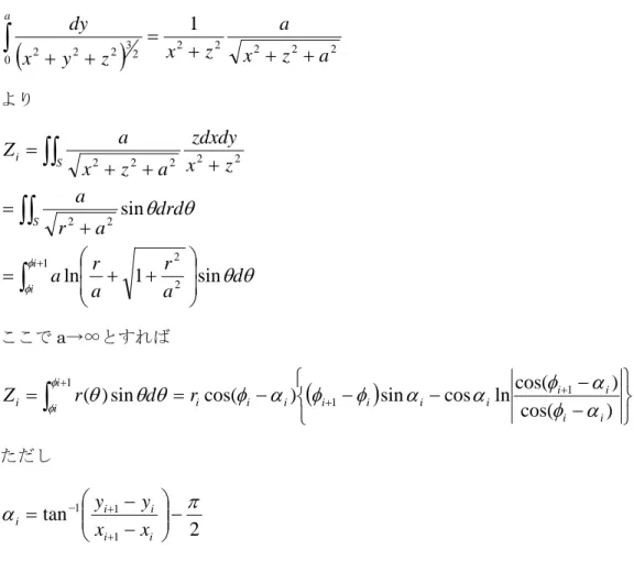
+ + + 断面線から端の長さがa である有限 2 次元モデルの計算式について考慮する。(
)
2 2 2 2 2 0 2 3 2 2 21
a
z
x
a
z
x
z
y
x
dy
a+
+
+
=
+
+
∫
よりθ
θ
θ
θ
φ φa
d
r
a
r
a
drd
a
r
a
z
x
zdxdy
a
z
x
a
Z
i i S S isin
1
ln
sin
1 2 2 2 2 2 2 2 2 2∫
∫∫
∫∫
+
+
+
=
+
=
+
+
+
=
ここでa→∞とすれば(
)
∫
+ + +
−
−
−
−
−
=
=
1 1 1)
cos(
)
cos(
ln
cos
sin
)
cos(
sin
)
(
i i i i i i i i i i i i i ir
d
r
Z
φ φφ
α
α
φ
α
α
φ
φ
α
φ
θ
θ
θ
ただし2
tan
1 1 1π
α
−
−
−
=
+ + − i i i i ix
x
y
y
Komazawa(1995)より 2 次元多層モデルの計算プログラム angmdl2.f 入力ファイル 重力データgravdata.txt 119 ← データ数 1 1.73774 -1473.8 12.426 ← NN, XD(km),H(m),G-obs(mgal) 2 3.96276 -1468.3 10.861 3 6.19107 -1537.8 7.485 入力モデルは下図。モデルパラメーターmodel.txt 3 2 1 ← lay(層の数)、ipol(トレンドの次数)、it(1=トレンドを計算する、0 =計算しない) 118 0.4 1 5000 ← lpnt(エッジの数)、dnl(密度差 mgal)、lex(1=オープン層、 0=クローズ層;p(1)=p(end)であるような層をクローズ層という)、aa(層の幅m) 1 1.73774 -1473.8 ← NN, XD(km),H(m) ・・・・・ 2222 ← ik(2222=層の終わり、3333=ファイルの終わり) 計算結果
ここから同様にモデルを微修正する。 ΔH(m)=(calcg-obsg) (mgal)/(2*3.14*6.67*0.001*Δρ(mgal)) を計算し、修正したい箇所に加える。ここで修正値が地形データより大きくなったら、そ の部分は地形データで置き換える。 Blakely の計算式を使ったモデルと少々違うのは当然のこと。 C→E へモデルを修正。 計算結果
両端の値はモデルの打切り誤差の影響なので、ここでは無視する。 更に修正を加える場合もあるし、この辺で良しとする場合もある。
プログラム
c 2-D Gravity Model program
c ver.1 with observed data c original Komazawa-san c modified RIE Morijiri c c - ang - common /ag/ag(500) common /xa/xa(500)/ya/ya(500) common /xb/xb(500)/yb/yb(500) c - iteration - common /gc/gc(500)/go/go(500) common /to/to(500)/rg/rg(500) common /xo/xo(500)/yo/h(500) common /xp/xp(500)/yp/d(500) common /xc/xc(500)/yc/dc(500) common /ite/iobs,den,ipol,it c - layers data - common /gl/gl(500,20) common /xl/xl(500,20)/yl/yl(500,20) common /lay/lay,lpnt(20),dnl(20),lex(20),ldpl(20),aa(20) c - - - data i2,i3/2222,3333/ c open(10,file='I:¥grav-DB¥model.txt',status='old') open(15,file='I:¥grav-DB¥gravdata.txt',status='old') open(30,file='I:¥grav-DB¥angresult.txt') c --- obs.pnt. input --- read(15,*) iobs m = 0 do 2 k=1, iobs read(15,*) nn,xd,hei,gobs m = m + 1
xo(m) = xd*1000 h(m) = hei go(m) = gobs 2 continue mw=m close(15) c c write(6,616)
c 616 format(1h ,'--- distance from origin ---') c write(6,603) (xo(i),i=1,mw)
c write(6,617)
c 617 format(1h ,'--- height data ---') c write(6,603) (h(i),i=1,mw) c write(6,618)
c 618 format(1h ,'--- observed gravity data ---') c write(6,603) (go(i),i=1,mw)
c if( mw .ne. iobs ) go to 3 c - - -
read(10,*) lay,ipol,it c - - -
write(6,601) iobs,lay,ipol,it
601 format(1h ,'iobs =',i5,5x,'lay no. =',i5/ & 1h ,'ipol=',i2,5x,'it =',i2) c
c +++++++++++++++++++++++++++++++++++++++ c +++ calculation of layers structure +++
c +++++++++++++++++++++++++++++++++++++++ c ***************************** c * l : layer's no. * c * lpnt: layer's points * c * dnl : layer's density * c ***************************** c if( lay .le. 0 ) go to 4
l = 0 11 l = l + 1
read(10,*) lpnt(l),dnl(l),lex(l),aa(l) k = 0 c >---> do 12 i=1,lpnt(l) read(10,*) ii,xd,yd k = k + 1 xl(k,l) = xd*1000 yl(k,l) = yd 12 continue c <---< read(10,*) inum
write(6,*) '83-inum ; ',inum if( k .ne. lpnt(l) ) go to 5 if( inum .eq. i2 ) go to 11 if( l .ne. lay ) go to 4 if( inum .eq. i3 ) go to 13 c >---> l-th layer data input >---> c --- calculation of layers structure ---> 13 continue
do 21 l=1,lay
lw = 10*( lpnt(l)/10 + 1 )
write(6,619) l,dnl(l),lpnt(l),lex(l),aa(l)
619 format(1h0,10x,'***',i2,'-th layer ***',5x,'den =',f6.2,5x, & 'lpnt =',i3,5x,'lex =',i2,5x,'width =',f8.1/)
write(6,606)
606 format(1h ,10x,'--- x(layer boundary) ---') write(6,603) (xl(i,l),i=1,lw)
write(6,607)
607 format(1h ,10x,'--- y(layer boundary) ---') write(6,603) (yl(i,l),i=1,lw) c - - - jpnt = lpnt(l) dnj = dnl(l) jex = lex(l) c jdpl = ldpl(l) aaj = aa(l)
c - - - call chg1(xo,xa) call chg1(h,ya) call chg2(xl,l,xb) call chg2(yl,l,yb) c --- l-th layer's values ---> call angleg(iobs,jpnt,dnj,jex,aaj) c <--- call chg3(ag,gl,l) c - - - write(6,608)
608 format(1h ,10x,'--- g(calculated values) ---') write(6,603) (gl(i,l),i=1,mw)
21 continue
c <--- calculation of layers structure --- do 15 i=1,iobs
gc(i) = 0. do 14 l=1,lay gc(i) = gc(i) + gl(i,l) 14 continue 15 continue write(6,615) write(6,603) (gc(i),i=1,mw) go to 8 c >---> 3 write(6,620)
620 format(1h ,'***** observed point(iobs) is error. *****') go to 310
4 write(6,621)
621 format(1h ,'***** layers number is error. *****') go to 310
5 write(6,622) l
622 format(1h ,'*****',i2,'-th layer points is error. *****') go to 310
c <---< 8 continue
c - - - call trend(ipol,it)
call stadev(iobs,gc,go) write(6,615)
615 format(1h0,5x,'--- calculated gravity ---') write(6,603) (gc(i),i=1,mw) c - - - do 88 i=1,mw write(30,*) xo(i),gc(i),go(i) 88 continue close(30) c ++++++++++++++++++++++++++++++++++++++++++++ 310 continue 600 format(1h0,5x,'---'/ / 1h ,5x,'line name = ',3a4/ / 1h ,5x,'---') 603 format(1h ,10f10.2)
605 format(1h ,11x,' mean depth = ',f10.2) 609 format(1h ,10(5x,5h---))
stop end
c ****************************** c angleg * two dimensional analysis * c * by angle integration * c ****************************** subroutine angleg(iobs,ipnt,den,iex,aa) common /ag/ag(500) common /xa/xo(500)/ya/yo(500) common /xb/xp(500)/yb/yp(500) c --- exterpolation of structure ---- call kyoku(xo,iobs,omin,omax) call kyoku(xp,ipnt,pmin,pmax) call kyoku(yo,iobs,ymin,ymax) xs = amin1(omin,pmin) xe = amax1(omax,pmax) rng = xe - xs
m = iobs n = ipnt + 6
if( iex .eq. 0 ) n = ipnt dm = 0. do 1 i=1,ipnt dm = dm + yp(i) 1 continue dmean = dm/float(ipnt) dpl=amin1(dmean,ymin) c if( idpl .eq. 0 ) dpl = 0. c if( idpl .ne. 0 ) dpl = dmean
write(6,601) iobs,ipnt,den,xs,xe,rng,dmean 601 format(1h0,15x,'angtal : iobs =',i4,3x, & 'ipnt =',i4,5x,'den =',f6.2/
& 1h ,15x,' : xs =',e12.4,3x,'xe =',e12.4,5x, & 'rng =',e12.4/
& 1h ,15x,' : mean depth = ',e12.4/) xs = xp(1) ys = yp(1) xe = xp(ipnt) ye = yp(ipnt) xp(ipnt+1) = xe + 0.5*rng xp(ipnt+6) = xs - 0.5*rng xp(ipnt+2) = xe + rng xp(ipnt+5) = xs - rng xp(ipnt+3) = xe + 4.*rng xp(ipnt+4) = xs - 4.*rng yp(ipnt+1) = ye yp(ipnt+6) = ys yp(ipnt+2) = 0.6*ye + 0.4*dpl yp(ipnt+5) = 0.6*ys + 0.4*dpl yp(ipnt+3) = dpl yp(ipnt+4) = dpl c --- c --- calculation of obs.pnt --- do 10 i=1,m
atl = 0. x0 = xo(i) y0 = yo(i) do 20 j=1,n x1 = xp(j) y1 = yp(j) k = j + 1 if( j .eq. n ) k = 1 x2 = xp(k) y2 = yp(k)
if( aa. eq. 0. .or. aa. eq. 99999. ) go to 11 atl = atl + den*sal(x0,y0,x1,y1,x2,y2,aa) go to 20
11 atl = atl + den*tal(x0,y0,x1,y1,x2,y2) 20 continue ag(i) = atl 10 continue c --- return end c *-*-*-*-*-*-*-*-*-*-*-*-*-*-* function tal(x0,y0,x1,y1,x2,y2) pai = 3.141593 yen = 2.*pai gg = 6.670e-3 rr1 = (x1-x0)**2 + (y1-y0)**2 rr2 = (x2-x0)**2 + (y2-y0)**2
if( rr1 .eq. 0. .or. rr2 .eq. 0. ) go to 100 r1 = sqrt(rr1) r2 = sqrt(rr2) pl = (x1-x0)*(y2-y0) - (x2-x0)*(y1-y0) sg = 1.0 if( pl .lt. 0. ) sg = -1. qh = phase(x2-x1,y2-y1) - 0.5*pai ph1 = phase(x1-x0,y1-y0) ph2 = phase(x2-x0,y2-y0)
phm = abs(ph2-ph1)
if( phm .eq. 0. ) go to 100
if( phm .gt. pai .and. phm .le. yen ) phm = yen - phm c1 = cos(ph1-qh) c2 = cos(ph2-qh) if( c1 .eq. 0. ) go to 100 ab = abs(c2/c1) alg = alog(ab) tt = r1*c1*( sg*phm*sin(qh) - alg*cos(qh) ) go to 200 100 tt = 0. 200 continue tal = 2.0 * tt * gg return end c *-*-*-*-*-*-*-*-*-*-*-*-*-*-* function sal(x0,y0,x1,y1,x2,y2,aa) pai = 3.141593 yen = 2.*pai gg = 6.670e-3 tt = 0. rr1 = (x1-x0)**2 + (y1-y0)**2 rr2 = (x2-x0)**2 + (y2-y0)**2
if( rr1.eq.0. .or. rr2.eq.0. ) go to 100 r1 = sqrt(rr1) ph1 = phase(x1-x0,y1-y0) ph2 = phase(x2-x0,y2-y0) qh = phase(x2-x1,y2-y1) - 0.5*pai pp1 = ph1 - pai pp2 = ph1 + pai if( ph2 .lt. pp1 ) ph2 = ph2 + yen if( ph2 .gt. pp2 ) ph2 = ph2 - yen if( abs(sin(ph2-ph1)) .lt. 0.0001 ) go to 100 c --- nn : division number --- nn = 16
if( abs( ph2-ph1 ) .gt. 0.50*pai ) nn = 51 c --- dh = ( ph2 - ph1 ) / float(nn-1) do 1 m = 1,nn phm = ph1 + float(m-1)*dh r = r1 * cos(ph1-qh) / cos(phm-qh) ra = abs( r / aa ) ab = abs( ra + sqrt( ra*ra + 1.0 ) ) alg = alog( ab ) sg = 1.0
if( m .eq. 1 .or. m .eq. nn ) sg = 0.5 c tt = tt + sg * dh * r * sin(phm) tt = tt + sg * dh * aa * alg * sin(phm) 1 continue go to 200 100 tt = 0. 200 continue sal = 2.0 * tt * gg return end c *-*-*-*-*-*-*-*-*-*-*-*-*-*-* function phase(px,py) pai = 3.141593
if( px .ne. 0. .and. py .ne. 0. ) go to 1 if( py .eq. 0. .and. px .ge. 0. ) ph = 0. if( py .eq. 0. .and. px .lt. 0. ) ph = pai if( px .eq. 0. .and. py .gt. 0. ) ph = 0.5 * pai if( px .eq. 0. .and. py .lt. 0. ) ph = 1.5 * pai go to 6
1 ph = atan(py/px)
if( px .lt. 0. ) ph = ph + pai
if( px .gt. 0. .and. py .lt. 0. ) ph = ph + 2.0*pai 6 phase = ph
return end
subroutine trend(ipol,it) common /equ/p(6,7),pn(6),q(6) common /gc/gc(500) common /go/go(500) common /to/to(500) common /rg/rg(500) common /ite/iobs common /xo/xo(500)/xc/xc(500)
if( ipol.ge.0 .and. ipol.le.5 ) go to 100 write(6,600)
600 format(1h0,' the value of ipol is exceptional. ') go to 110 100 continue call kyoku(xo,iobs,omin,omax) rng = 3.*(omax-omin)/float(iobs) c - - - jpol = ipol + 1 do 1 i=1,6 pn(i) = 0. do 1 j=1,6 1 p(i,j) = 0. c >- - - do 2 i=1,iobs x = xo(i)
sa = go(i) - ( gc(i) + rg(i) ) q(1) = 1.
if( ipol .eq. 0 ) go to 4 do 3 k=1,ipol 3 q(k+1) = x*q(k) 4 continue c - - - - do 5 l=1,jpol pn(l) = pn(l) + sa*q(l) do 5 j=1,jpol 5 p(l,j) = p(l,j) + q(l)*q(j) 2 continue
c <- - - call matrix(jpol) write(6,603) (pn(i),i=1,6) 603 format(1h0,'trend : a(0)=',e12.3,3x,'a(1)=',e12.3,3x, / 'a(2)=',e12.3,3x/ / 1h ,' a(3)=',e12.3,3x,'a(4)=',e12.3,3x, / 'a(5)=',e12.3) do 6 i=1,iobs x = xo(i) q(1) = 1.
if( ipol .eq. 0 ) go to 8 do 7 k=1,ipol 7 q(k+1) = x*q(k) 8 continue gx = 0. do 9 j=1,jpol 9 gx = gx + pn(j)*q(j) to(i) = gx + rg(i)
if(it .eq. 1) gc(i) = gc(i) + to(i) 6 continue 110 return end c ******************************* subroutine matrix(iv) common /equ/p(6,7),pp(6),q(6) dimension m(6) ih = iv + 1 do 41 i=1,iv m(i)=i 41 continue do 15 i=1,iv p(i,ih) = pp(i) 15 continue do 1 i=1,iv if( p(i,i).ne.0. ) go to 5 do 6 j=i,iv
if( p(j,i).ne.0. ) go to 8 6 continue go to 12 8 do 7 k=1,ih b = p(j,k) p(j,k) = p(i,k) p(i,k) = b 7 continue go to 5 12 do 9 j=i,iv if( p(i,j).ne.0. ) go to 10 9 continue go to 13 10 ic = m(i) m(i) = m(j) m(j) = ic do 11 k=1,iv b = p(k,j) p(k,j) = p(k,i) p(k,i) = b 11 continue 5 w = p(i,i) do 2 j=1,ih p(i,j) = p(i,j)/w 2 continue do 3 k=1,iv if( k.eq.i ) go to 3 s = p(k,i) do 4 l=1,ih p(k,l) = p(k,l) - s*p(i,l) 4 continue 3 continue 1 continue do 51 i=1,iv ip = m(i) pp(ip) = p(i,ih)
51 continue go to 14 13 continue write(6,600)
600 format(1h ,'matrix : calculation is impossible.') 14 continue return end c ******************************** subroutine stadev(m,gc,go) dimension gc(1) dimension go(1) dimension gs(500) su = 0. do 1 i=1,m s = gc(i) - go(i) 1 su = su + s sa = su/float(m) do 2 i=1,m 2 gs(i) = gc(i) - sa su = 0. do 3 i=1,m s = gs(i) - go(i) 3 su = su + s*s su = su/float(m-1) sd =sqrt(su) write(6,600) sa,sd write(30,600) sa,sd
600 format(1h ,'stadev : mean difference =',f12.5/ / 1h ,' : standard deviation =',f12.5) return end c ******************************** subroutine kyoku(a,m,rmin,rmax) dimension a(1) rmin = a(1)
rmax = a(1) do 1 i=1,m ad = a(i) if( ad .lt. rmax ) go to 2 rmax = ad go to 1 2 if( ad .gt. rmin ) go to 1 rmin = ad 1 continue return end c ****************************************** subroutine gxysa(xor,xen,gmin,gmax,smin,smax) common /ite/m common /gc/gc(500)/go/go(500)/to/to(500) common /xo/xo(500)/yo/h(500) call kyoku(xo,m,omin,omax) xor = omin xen = omax call kyoku(h,m,hmin,hmax) smin = hmin smax = hmax call kyoku(go,m,omin,omax) call kyoku(gc,m,cmin,cmax) call kyoku(to,m,tmin,tmax) gmin = amin1(omin,cmin,tmin) gmax = amax1(omax,cmax,tmax) return end c ****************************************** subroutine glxymm(xlor,xlen,glmin,glmax,slmin,slmax) common /ite/m common /lay/lay,lpnt(20),dnl(20),lex(20) common /gl/gl(500,2) common /xl/xl(500,2) common /yl/yl(500,2)
dimension a(500)
if( lay .eq. 0 ) go to 10 do 1 l=1,lay
call chg2(gl,l,a)
call kyoku(a,m,amin,amax) if( lay .eq. 1 ) glmin = amin if( lay .eq. 1 ) glmax = amax if( amin .lt. glmin ) glmin = amin if( amax .gt. glmax ) glmax = amax 1 continue 10 continue call tpbtl(xl,xlor,xlen) call tpbtl(yl,slmin,slmax) return end c ****************************************** subroutine tpbtl(gl,glmin,glmax) common /lay/lay,lpnt(20),dnl(20),lex(20) dimension gl(500,20),a(500)
if( lay .eq. 0 ) go to 10 do 1 l=1,lay
call chg2(gl,l,a) jpnt = lpnt(l)
call kyoku(a,jpnt,amin,amax) if( lay .eq. 1 ) glmin = amin if( lay .eq. 1 ) glmax = amax if( amin .lt. glmin ) glmin = amin if( amax .gt. glmax ) glmax = amax 1 continue 10 continue return end c *********************** subroutine chg1(a,b) dimension a(500),b(500) do 1 i=1,500
1 b(i) = a(i) return end c ************************* subroutine chg2(a,m,b) dimension a(500,20),b(500) do 1 i=1,500 1 b(i) = a(i,m) return end c ************************* subroutine chg3(a,b,n) dimension a(500),b(500,20) do 1 i=1,500 1 b(i,n) = a(i) return end