Advanced Safety Vehicle (ASV) Technology Driver Support System Monitor using Three Onboard Camera

Monitor using Three Onboard Camera

Stephen Karungaru

_{Tomohiro Ishino}

Kenji Terada

(Received August 1, 2017, revised October 8, 2017)

Abstract: This paper presents the development of safety driving support system using 3 onboard cameras. One camera monitors the driver to determine the driver ’s current gaze and the other is a front camera that detects pedestrians, running lane and vehicles in front. The rear camera detects pedestrians and approaching vehicles. The pedestrians and vehicles are detected using a specially trained HOG/Adaboost system. Lane detections uses edge detection and RANSAC. Information from the 3 cameras is then used to determine whether a situation is dangerous enough to warrant warning the driver. We have conducted experiments and the results confirm that this system has the potential to support automatic driving

Keywords: HOG feature value, human detection, vehicle detection, RANSAC, Adaboost

1. Introduction

In recent years, the number of occurrences of traffic ac-cidents in Japan is decreasing due to progress and appli-cation of intelligent transportation systems [1]. However, more than 500,000 traffic accidents still occur each year, and the number of traffic accident deaths since 2005 has been steadily increasing to over 4,000 people every year. Moreover, the number of occurrences of traffic accidents by violation of laws and regulations by drivers (first parties) remains greater than that of mopeds. Of the causes, safety non-confirmation accounts for about 30.4%, inattentiveness operation about 16.7%, and vigorous and unconsciousness about 11.5%. These 3 violations account for over 58% of total accident causes. It can be confirmed that the causes of those accidents are the following law violations; uncon-firmed safety, negligence, erroneous confirmation of safety, etc. Therefore, driver’s carelessness is a main cause. More-over, various kinds of road conditions occur due to road sit-uations, for example, changing of lanes, vehicles in front and behind, intersections, sidewalks, etc. It is therefore also paramount to grasp the numerous situations during driving and to confirm the safety.

Several driver support systems have already been pro-posed under the Advanced Safety Vehicle (ASV) technol-ogy program. These include the LiDAR [2] and Mobileye [3]. The LIDAR system uses an infrared camera attached on the top of the vehicle. It can capture a surround image and calculate distance to objects. However, its drawbacks in-clude difficulty in installation and high cost. The mobileye system uses one front dashboard camera to capture the

dis-∗_{Corresponding author: karungaru@tokushima-u.ac.jp} †_{Tokushima University,}

2-1 Minami Josanjima, 770-8506, Tokushima, Japan.

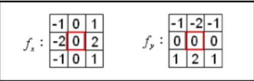
Figure 1: Sobel operator

tance to objects in front of the vehicle. Although it is easy to install and inexpensive, its range of operation is narrow and therefore, not very effective for driver support.

In this paper, we propose a system similar to Mobileye but set up three cameras inside the vehicle to capture the front, the back, and the driver ’s face, and propose a more effective driving support system. The system uses HOG fea-tures and Adaboost for person and vehicle detection, detects driving lanes, driver features like nostril and pupils. This in-formation is combined to design the driver support system. The system first detects the lanes from the image acquired from the front and rear cameras. Subsequently, objects such as people and vehicles are detected using Adaboost and HOG feature quantities, and the lane of the host vehicle is also determined. We then detect the nostrils and pupils from the image acquired from the internal camera and use the de-gree of separation to judge the gaze direction of the driver. The information is used to support the driver.

The following sections will explain each part of the pro-posed method in details. Results of experiments and discus-sions are presented before concluding.

2. Lane Detection

2.1 Edge Extraction After image capture, as a pre-processing step, edge detection is performed on the im-age. There are various operators for edge detection, among which the Sobel operator can best detect darker edges. We

Figure 2: Edge detection result

choose this filter in this work. However, white and orange lines existing on the road surface are thin, and there are cases where it is difficult to capture the color change within the asphalt surface. In addition, from the brightened image, the orange line has a feature that makes it difficult to capture the color change as compared with the white line. For this reason, edge detection is performed separately using the So-bel operator from the R, G, and B channels of the acquired image, and those having the highest edge intensity among them are detected as edges.

Fortunately, the white lines used to determine the driving lane region exists only on the road surface. Therefore, by limiting the range of edge detection, we aim to eliminate noise that can be detected from artifacts such as buildings along side roads and pedestrian bridges that are likely to have linear edges. This step can greatly shorten the overall processing time. Consequently, the range to be detected is only the one to two-thirds area from the top of the captured region surroundings the vehicle. Figure 1 shows the Sobel operator, and Fig. 2 shows the edge detection result.

From the edge detection images, we remove noisy edges for white line detection. There are many edges other than the white lines, such as small edges existing on the road surface, white line edges of the adjacent lane, edges such as in front and oncoming cars, and curbstones on the de-tected edges. We aim to improve the accuracy of detection of white lines and the detection speed by eliminating these edges as noise. One useful feature of the small edges exist-ing on the road surface is small edge strength. Therefore, when the strength of any edge is 80 or less, it is removed as noise. However, the white line edges of the adjacent lane, the edges of the front and the oncoming car, the curb stone, etc. will still remain. Fortunately, the edges other than the white line of the driving lane has a characteristic that the gradient direction has a value close to 270 degrees, so noise can also be reduced using the gradient direction. Only the edges that satisfy the condition shown in expres-sions (1) and (2) are used for white line detection with|∇ f | andθ representing the edge strength and gradient direction respectively. Figure 3 shows the edge detection image with noise removed.

|∇ f | ≥ 80 (1)

{

200< θ < 260

300< θ < 360 (2)

Figure 3: Noise removal result

(a) Edge detection (b) Line detection result

Figure 4: Line detection result

2.2 White line detection We aim to detect two straight lines from the detected edges. RANSAC [4] method is applied for straight line detection. RANSAC is a robust model generation method based on random sam-pling. Its concrete procedures are described below.

1. Randomly sample the data on the edge.

2. Select two points randomly from the sampled data. 3. Find the parameters of the straight line passing through

the two selected points.

4. Vote on the number of data that exists within the fixed threshold of the obtained straight line.

5. Save the number of voted data and the two selected points.

6. Repeat from step 2.

This operation is performed 1000 times to detect two straight lines with positive and negative slopes and having largest data. Figure 4 shows an example of straight lines detection using RANSAC.

Since there are cases where the two straight lines detected are not white lines, white line judgment is performed on those straight lines. When capturing the image using the front and the rear of the vehicle from the on-board camera, the white line is often straight. Therefore, the intersection of the straight lines on the white line exists near the van-ishing point in the center of the image. In addition, when a correct white line cannot be detected, the angle formed by the straight line on the white line has a value close to 180 ° or 0 ° . Therefore, the white line is detected using the angle formed by the intersection point of the straight line on the white line.

Let the area sandwiched by white lines be the traffic lane area, the left side of the white line detected on the left side

Figure 5: Lane area

of the image will be the left lane area, and the right side of the white line detected on the right side of the image will be the right lane area. Let the intersection point of the straight line on the white line be Lx, Lyand the angle formed be Lθ.

If conditional expressions 3 and 4 are satisfied, the detected straight line will be a white line.

{

240< Lx< 420

180< L_y< 310 (3)

10< L_θ< 110 (4)

2.3 Dotted Line determination In order to classify the lane that the host vehicle is on, the detected white and orange lines are classified as straight or dotted. Lane clas-sification is performed by a combination of a straight white and dotted lines. If the left white line is straight and the right white line is dotted, the running lane will be the left-most lane. Also, if the left white line is a dotted line and the left white line is a straight line, the running lane is the rightmost lane. If both are dotted or straight lines, it is the central lane.

For the determination of the dotted line and the straight line, the existence ratio E of the number of pixels of the edge present on the detected white line is used. Let the distance from the point of intersection of the straight lines to the edge of the vehicle be D and the number of pixels of the edge on the detected white line be X. The existence rate E of the white line is calculated by the formula 5. When the existence ratio E of the white line is 0.3 or more, the line is straight, otherwise it is a dotted (Fig. 6).

E= X

D (5)

3. People and vehicle object detection

3.1 HOG Feature Value In this work, images are captured using a USB camera mounted on the vehicle. Therefore, it is difficult to accurately detect vehicles using background difference, etc. Hence, the HOG feature quan-tity is used to capture the characteristics of the vehicle.

We introduce HOG feature quantities to detect vehicles from the captured images [5]. In order to obtain the HOG feature amount, we extract the HOG feature quantity using a cell size set as 8× 8 pixels, the size of the block as 3 × 3 cells, and the histogram of the edge to be created hav-ing nine bins with 20 ° increments. Equations (6) and (7)

Figure 6: White line existence rate

Figure 7: Original image

are used for the gradient direction and strength calculation respectively. Equation 9 is used to normalize feature quan-tities for a certain nthblock.

m(x, y) = √ fx(x, y)2+ fy(x, y)2 (6) θ(x, y) = tan−1 fx(x, y) f_y(x, Y) (7) { fx(x, y) = L(x + 1, y) − L(x − 1, y) f_y(x, y) = L(x, y + 1) − L(x, y − 1) (8)    m(x, y) : Gradientstrength θ(x, y) : Gradientdirection L(x, y) : Luminancevalue v(n) =_√(∑ v(n) Q·N k=1v(k)2 ) + 1 (9)    v(n) : Featurevalue Q : Numberofcellsinblock N : Gradientdirectionnumber

Figure 8 shows the result of calculating and converting the HOG feature amount for the image shown in Fig. 7. 3.2 Adaboost The HOG feature quantity is learned using Adaboost [6]. Adaboost is a machine learning algo-rithm that can learn with less data. It calculates the sum of the product of the output of weak classifiers hiallocated

to the cell in the search window and the reliability αiand

discriminate between human and non-human in the input image. The expression of the weak classifier hiis shown in

Figure 8: HOG

expression 10. The expression of the reliabilityαiis shown

in the expression 11. hi(y, x) = { 1 : hog(y, x) ≥ th −1 : hog(y, x) < th (10) th : Maximumseparationthreshold

hog(y, x) : TheHOGfeatureamount (y, x) oftheimagecell

αi= loge ( 1− ei ei ) · 0.5 (11) ei: Incorrectanswerrateofweakclassifiers

The weight of the learning sample is updated by the cal-culated reliability, class label, and response of the weak classifier. The formula for updating the weight is shown in Equation 12. The denominator of Eq. 12 is the sum of the weights of the samples. We also normalize the weights.

Dt₊₁(i)=

Dt(i) exp (−αtytht(i))

∑N

i=1Dt(i) exp (−αtytht(i))

(12)

4. Driving lane determination

We determine the traffic lanes of detected vehicles and lo-cation of people using information acquired by lane detec-tion, human and vehicle detection. In the case where the midpoint of the lower side of the circumscribed quadran-gle of the detected person or vehicle exists in the traveling lane area, it is assumed that the front object is the preceding vehicle, and if it is the rear image, the following vehicle. 5. Nostril and pupil detection

In this work, the position and size of the face greatly differs for each subject depending on the vehicle, the sitting height, the position of the chair, etc. Therefore, parameters of the face search region are set for each subject. The face search area is set so that its upper end is above the eyebrow, the lower end is near the jaw and the horizontal width is about 3 times the eye width in a front facing state.

For the purpose of speeding up the processing performed in this part, processing is performed on the luminance image already obtained. Next, in order to improve the accuracy of nostril and pupil detection and to reduce the processing speed, the detection region is limited. Features of nostrils

(a) Original image (b) Search area extraction result

Figure 9: Nostril Search Area

Figure 10: Nostril detection filter

Figure 11: Eye detection filter

and pupils are characterized by low brightness values re-gardless of changes in sunshine. For this reason, we use only the area of the face search area whose luminance value is 70 or less. Figure 9 shows the nostril search area.

Next, detection of the nostrils or pupils is performed us-ing the degree of separation. In the interior of the vehicle, the brightness fluctuates due to the influence of sunshine and it is difficult to extract skin color. For this reason, sight line classification is carried out using a region such as a nos-tril or pupil where there is little change in color due to varia-tion in brightness. When detecting the nostrils, detecvaria-tion is performed using the nostril detection filter in Fig. 10. When detecting the pupil, use the pupil detection filter in Fig. 11. The pupil detection area is from the midpoint of the nostril up to a fifth of the height of the face search area.

Calculation of the degree of separation is performed us-ing the outer and the inner regions both in the nostrils and pupils. At first we find the degree of separation between the red and the blue regions. The obtained degree of separa-tion is calculated as a normalized value and is close to the maximum value 1.0 when the two regions are completely separated. On the other hand, when it is not separated, it approaches the minimum value 0.0. Equation 13 shows the equation for obtaining the degree of separationµ.

η = σ 2 b σ2 T (13) σ2 b= n1(m1− m)2+ n2(m2− m)2 σ2 T = ∑ x∈C (x− m)2

Figure 12: W

Figure 13: Z

Figure 14: X, Y

For the nostril detection, two maximum values of the de-gree of separation calculated from the nostril search region are used. However, there are cases where the detected nos-trils are double-counted by selecting two maximum values. Therefore, when the maximum value of the degree of sepa-ration is detected, nostrils are not detected from the region less than 5 pixels in radius.

6. Gaze direction determination

In this work, we set the position and size of face in advance and use it to classify the line of sight. Let W be the width of the face, Y the distance in the vertical direction from the co-ordinates obtained by shifting from the nostril horizontally and vertically by one-sixth of W to the pupil, and X the dis-tance in the lateral direction. Figures 12, 13, and 14 shows W, Z, X, and Y.

Eye direction widthsθx, andθyare calculated using

ex-pression (14). Let Z be the distance in the horizontal di-rection from the center of the face area to the midpoint of the nostril. The orientationθ of the face in the horizontal direction is calculated by the formula (15).

θy= arctan2Y_W, θx= arctan

2X

W (14)

ward, it is determined that the right or the left mirror is being viewed. When facing the front and the pupil is upward, it is judged that the subject is looking at the room mirror. If it is judged that the subject is looking at the front and if the pupil is facing the right or left, the subject is watching the right lane or sidewalk or the left lane.

We classify our eyes using conditional expressions (16), and (17).     Roommirror : 75< θ < 110, 30 < θx< 70, 85, θy Rightmirror : 90 < θ, 101 < θx, 102 < θy Le f tmirror :θ < 80, θx< 70, 102 < θy Front : 80< θ < 130 (16)    Le f tLane : 75< θx< 90, θy> 94 DrivingLane : 90 < θx< 100, θy> 94 RightLane : 100 < θx< 110, θ_y> 94 (17)

7. Dangerous object determination

We determine the danger posed by an object captured by the cameras using the distance between the detected object and the host vehicle.

7.1 Approach determination In this section, we will describe approach determination of nearby vehicles and people to establish the objects that the driver must pay at-tention to while driving.

We estimate the distance (in pixels) change between the host vehicle and the surrounding vehicles by measuring the distance between them. In the case of a vehicle on the right or left adjacent lane, the distance from the nearest point on the white line detected from the center of gravity of the de-tected vehicle to the lower end of the image along the white line is the distance to the vehicle. In the case of the preced-ing vehicle existpreced-ing in the drivpreced-ing lane, the distance from the center of gravity of the vehicle to the lower end of the image is the distance to the vehicle.

The distance acquisition of the vehicle is performed in every frame, and when the acquired distance decreases from the previous frame, the approach count of the vehicle is decremented by one. Also, if not approaching, increment the approach count by+1. When the approaching count of the vehicle falls below−3, it is determined that the vehicle is approaching.

7.2 Warning judgment The monitoring and warning determination are made to judge whether or not the driver is performing safety confirmation using the information on the approaching determination result of the gaze direction.

First, if the driver is not gazing at the vehicle when ap-proaching is determined for the vehicle detected on the left or the right lane, it is judged that the driver is not performing safety confirmation and the warning is sounded. In addition,

the driver and a camera oriented to face the driver on the dashboard are installed to capture the data required.

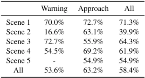
The data set used for HOG vehicle and human detec-tion is from INRIA Person Dataset [7] and CBCL Pedes-trian Database [8] respectively. The driver-facing camera is oriented such that the driver ’s face is at the center of the frame. Also, cameras capturing the front and rear of the vehicle are installed so to shoot above the position of approximately 235 pixels. The image size is 640× 480. Three cameras with one laptop are used. Same numbers are assigned to images taken at the same time and saved. Pro-cessing is performed on the saved three sets of consecutive number images. Shooting time was done during the day. 8.2 Experiment result accuracy This section shows the accuracy of the experiments. Table 1 shows lane deter-mination results, Table 2 shows gaze judgment, and Table 3 shows dangerous object judgment.

Table 1: Lane determination

Left lane Driving Right lane all Scene1 - 57.2% 89.4% 73.3% Scene2 97.4% - - 97.4% All 97.4% 57.2% 89.4% 91.3%

Table 2: Gaze determination All Subject A 86.9% Subject B 79.3% All 82.3%

Table 3: Dangerous object determination Warning Approach All Scene 1 70.0% 72.7% 71.3% Scene 2 16.6% 63.1% 39.9% Scene 3 72.7% 55.9% 64.3% Scene 4 54.5% 69.2% 61.9% Scene 5 - 54.9% 54.9% All 53.6% 63.2% 58.4%

8.3 Lane determination In scene 1, processing was performed on a scene in which the left white line is straight and the right white line is a dotted. In scene 1, it was judged that the driving lane was the left end for 380 frames out of

Figure 15: Right lane determination image

Figure 16: Room mirror decision image

390 frames processed, and it was possible to obtain a highly accurate result, so it can be said that generally good results were obtained.

In scene 2, processing was carried out for scenes where the white line on the left side is dotted, the white line on the right side runs on a straight lane, and the white lines on both sides are straight. In scene 2, among the 238 frames processed, the traveling lane was judged to be the center for 71 frames out of the 124 frames for the center lane when the left and right white lines were straight. In addition, the driving lane was judged to be the right end for 102 frames out of the 114. Generally good results were obtained. The cause of erroneously determining of the central lane as the rightmost lane is that the white line on the left was hidden and the white line existence ratio decreased as it approached the preceding vehicle at the time of signal change wait. In order to improve the accuracy, it is necessary to determine whether or not the white line is occluded by a vehicle, and to add exception processing accordingly.

The right lane determination result is shown in Fig. 15. 8.4 Fixation judgment In gaze determination exper-iments, experiments were conducted on two subjects, A and B.

For subject A, we handled the scene where the driver gazes to the front, right front, right, driving mirror and right side mirror. For subject A, the driver’s gaze direction was judged to be frontal for 930 frames out of the 1225 frames (for which the driver was facing the front for 1002 frames). In addition, the driver’s gaze direction was judged to be right-front for 64 out of the 74 frames. Also, the driver’s gaze direction of the driver was judged to be the right side

gazed at the front, the driving mirror, the right side mir-ror, and the left side mirror. The driver’s gaze direction was determined to be frontal for 180 frames of 194 frames. In addition, the driver’s gaze direction was judged to be the driving mirror for 10 of the 16 frames. In addition, the driver’s gaze direction was judged to be the right side mir-ror for 10 of the 10 frames. Also, the driver’s gaze direction was judged to be the left side mirror for 7 of the 10. In addi-tion, the driver’s gaze direction was judged to be rightward for 5 of 7 frames. Good results were generally obtained for the front and right mirrors. There was a case that the gaze direction was erroneously determined as the front when the driver was looking at the room mirror. It is thought that erroneous judgment occurred because the feature looking at the front mirror is similar to the room mirror, the angle calculation method of the current face in the horizontal di-rection and the angle calculation of the eye. Therefore, it is necessary to examine features that are more likely to cap-ture changes in eye direction.

Fig. 16 shows the room mirror determination result. 8.5 Dangerous object determination In scene 1, processing was performed on the frames that include a pedestrian. It was possible for the driver to approach the pedestrian for 8 of the 11 frames. In addition, the driver was warned about the pedestrian in 7 of 10 frames. Errors occurred when detecting the person. It can be considered that a detection method corresponding to a change in size is necessary.

In scene 2, processing was carried out for a scene with an overtaking car and a passing bicycle. For the bicycle, the driver gazed at it for 9 of the 13 frames. Also, we were able to warn of the bicycle 6 of the 11.

Also, we made a decision on the oncoming vehicle. The driver gazed at the oncoming vehicle for 7 of the 23 frames. Also, it was not possible to make any judgment for 14 of 17 frames after passing the oncoming vehicle. It is necessary to improve the method so that smaller and large vehicles can be detected.

In scene 3, the vehicle being overtaken by the motorcy-cle at the intersection was processed. An accuracy of 12 of 19 frames was achieved. Also, it was possible to de-termine the approach of the motorcycle for 6 of 36 frames when the driver focused on the motorcycle. We could not detect the motorcycle because the approach determination could not be made after being overtaken. It seems that the detection failed because the side of the motorcycle was re-flected. In order to cope with it, it is necessary to create a learning image corresponding to the orientation of a person or a motorcycle.

In scene 4, processing was carried out for a scene that included an oncoming vehicle on a two-lane road. An

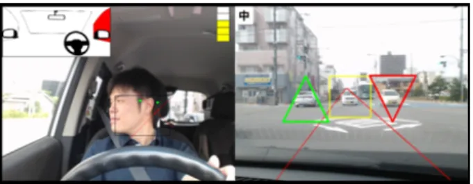
ac-Figure 17: Warning judgment

curacy of 28 of 51 was achieved. In many cases, approach determination cannot be made when detecting an oncoming vehicle at a short distance. Although the vehicle is moving towards the lower end on the image, the area where the vehi-cle is detected does not follow the movement of the vehivehi-cle and the upper part of the vehicle is detect. It is necessary to improve detection of vehicle movement.

In scene 5, processing was performed for a scene when entering an intersection in front of an opposite car and turn-ing right. An accuracy of 248 of 443 frames was achieved. In addition, when the driver was looking at the right, it was possible to trigger a warning of the oncoming vehicle ap-proaching for 16 of the 22 frames. Also, after the oncoming car passed, it was possible to make a decision for 127 of 194 frames away from the vehicle. The warning system ob-tained generally good results.

A warning determination result is shown in Fig. 17. 9. Conclusion

In this paper, we proposed driver support system using 3 on board cameras. We capture the driver, the vehicle in front and behind using the 3 cameras.

After edge detection, the RANSAC method is used to ex-tract straight lines. We detect the presence of a person of vehicle using HOG feature quantity and Adaboost. We also monitored the driver by detecting nostrils and pupils and judging gaze direction.

Experimental results confirmed that we can detect people and vehicles, estimate gaze direction, and detect hazardous objects using USB cameras during the day.

In future, we need to deal with dark scenes such as nighttime, tunnels, etc. In addition, when the driver wears glasses or sunglasses, it is necessary to improve the detec-tion method because of reflecdetec-tion of light by the lens. More-over, the detection of the pupil cannot be performed when the lens frame and pupil overlap. Finally, in order to put the system into practical use, it is necessary to improve pro-cessing speed using GPU or multithread propro-cessing.

References

[1] National Police Agency Traffic Bureau: “The Situation of the traffic Accidents Occurrence in 2015” http://www.e-stat.go.jp/SG1/estat/List.do?lid=000001150496 (2016/12/19, Japanese)

[2] Velodyne LiDAR HDL-64E obstacle detection sensor, http://velodynelidar.com/hdl-64e.html (Feb,

[5] N. Dalal and B.Triggs, “Histogram of Oriented Gradients for Human detection”, Proc. of CVPR 2005, Vol.1 pp.886-893, 2005

[6] Y. Freund and R. E. Schapire, “A decision-theoretic gener-alization of on-line learning and an application to boosting”,

Journal of Computer and System Sciences, Vol.55, No.119,

1997. DOI:10.1006/jcss.1997.1504

[7] LEAR group. “INRIA Person Dataset”. http://pascal. inrialpes.fr/data/human/(2016/12/19)

[8] MIT “CBCL Pedestrian Database”, http://cbcl. mit.edu/cbcl/software-datasets/CarData.html (2016/12/19)

Stephen Karungaru(Non-member) received a PhD in Information System Design from the Department of information science and Intelli-gent Systems, University of Tokushima in 2004. He is currently an associate professor in the same department. His research interests include pat-tern recognition, neural networks, evolutionary computation, image processing and robotics. Ishino Tomohiro(Non-member) received a master’s degree Information System Design from the Department of information science and In-telligent Systems, University of Tokushima in 2017.

Kenji Terada(Non-member) received the doctor degree from Keio University in 1995. In 2009, he became a Professor in the Department of Information Science and Intelligent Systems, University of Tokushima department. His research interests are in computer vision and image processing. He is a member of the IEEE, IEEJ, and IEICE.