Temperature Dependence of Magnetically Active Charge Excitations in Magnetite across the Verwey Transition
4
0
0
全文
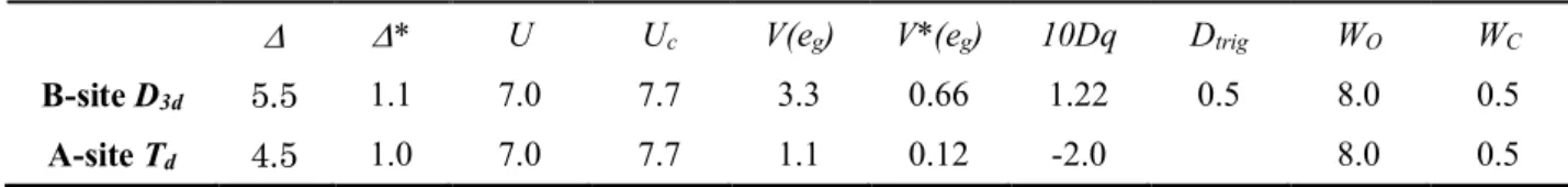
(2) C. Extended impurity Anderson model calculations We used the extended impurity Anderson model with full multiplets including a well-screened feature from the electronic state near EF to describe the spectra. The Slater integrals and the spin orbit coupling constants are calculated by Hartree-Fock code and are scaled down to 80% and 92%, respectively. The parameter values (in eV) are summarized in Table. S1. The parameters used in the calculations are: on-site Coulomb repulsion U, the attractive core-hole potential Uc, the charge transfer energy ∆, the crystal field 10Dq, the trigonal crystal field Dtrg in the B-site, Fe3d – O2p hybridization V(eg). For the hybridization, we use the relations: V(t2g)=√3V(eg) for Td symmetry and V(eg)=– 2V(a1g)=–2V(eg’) for D3d symmetry, respectively. We allow the 3d-band hybridization to be reduced by a factor RC (= 0.8) in the presence of the core hole and enhanced by a factor 1/RV (= 1/0.9) in the presence an extra 3d electron. We introduce the state C on the top of valence band and define the parameter: ∆* - the charge transfer energy between Fe 3d and C. An effective coupling parameter V*, for describing the interaction strength between the Fe 3d and coherent state is introduced, analogous to the Fe3d - O2p hybridization. We assume rectangular bands for O2p and coherent state C of width WO and WC, respectively. The precise XRD studies indicate the existence of small charge modulation below Verwey transition.[2-4] For example, Blasco et al. have shown ten different environments in the octahedral B-site, resulting ten different valences between 2.53 and 2.84. The valences of Fe(B1a), Fe(B1b'), Fe(B4'), Fe(B3) iron atoms were approximately 2.5 and the valences of Fe(B4), Fe(B1b) were about 2.7. The remaining B-site Fe atoms show more than 2.8 valences. Therefore, three types of parameter sets (i.e. Fe2.4~2.5+-like, Fe~2.7+-like and Fe2.8~2.94+-like) were used for the B-sites in the present calculations.. Table S1.. Estimated parameter values for high and low temperature phases of Fe3O4. High temperature phase (in eV) ∆. ∆*. U. Uc. V(eg). V*(eg). 10Dq. Dtrig. WO. WC. B-site D3d. 5.5. 1.1. 7.0. 7.7. 3.3. 0.66. 1.22. 0.5. 8.0. 0.5. A-site Td. 4.5. 1.0. 7.0. 7.7. 1.1. 0.12. -2.0. 8.0. 0.5. 2.
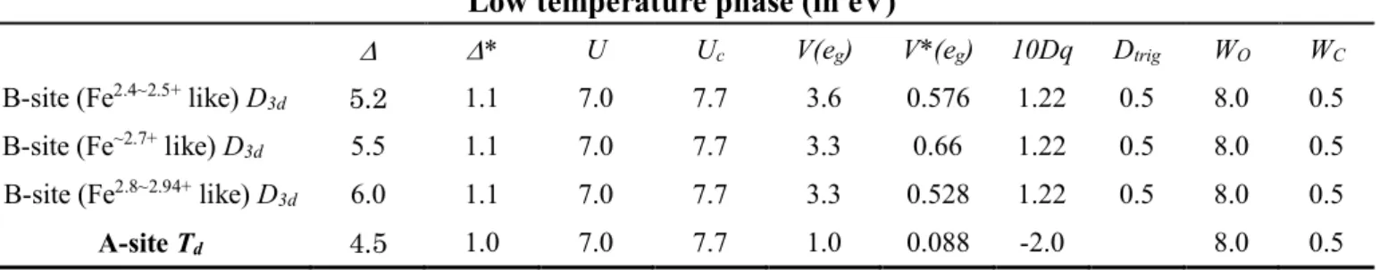
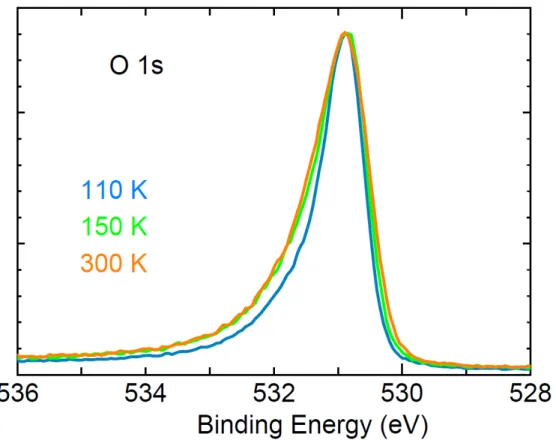
(3) Low temperature phase (in eV) 2.4~2.5+. B-site (Fe. like) D3d. B-site (Fe~2.7+ like) D3d 2.8~2.94+. B-site (Fe. like) D3d. A-site Td. ∆. ∆*. U. Uc. V(eg). V*(eg). 10Dq. Dtrig. WO. WC. 5.2. 1.1. 7.0. 7.7. 3.6. 0.576. 1.22. 0.5. 8.0. 0.5. 5.5. 1.1. 7.0. 7.7. 3.3. 0.66. 1.22. 0.5. 8.0. 0.5. 6.0. 1.1. 7.0. 7.7. 3.3. 0.528. 1.22. 0.5. 8.0. 0.5. 4.5. 1.0. 7.0. 7.7. 1.0. 0.088. -2.0. 8.0. 0.5. D. The details of the line-shape analysis of the temperature-dependent valence band PES Following the analysis by Kobayashi et al.[5], we have performed the same type of line-shape analyses for the temperature dependent valence band PES of single crystal Fe3O4. For the low temperature insulating phase, the line-shape was assumed to be of the form 𝐼𝐼 (𝐸𝐸𝐵𝐵 ) = 𝑎𝑎1 (𝐸𝐸𝐵𝐵 − 𝐸𝐸0 )𝜃𝜃(𝐸𝐸𝐵𝐵 − 𝐸𝐸0 ) in order to represent the finite gap 𝐸𝐸0 , where. θ(𝐸𝐸𝐵𝐵 − 𝐸𝐸0 ) is the step function. In the high temperature metal phase, we assumed. 𝐼𝐼 (𝐸𝐸𝐵𝐵 ) = (𝑎𝑎1 𝐸𝐸𝐵𝐵 + 𝑎𝑎0 )𝑓𝑓(𝐸𝐸𝐵𝐵 , 𝑇𝑇), where 𝑓𝑓(𝐸𝐸𝐵𝐵 , 𝑇𝑇) is the Fermi-Dirac distribution function at T. a0 and a1 were treated as adjustable parameters. E.. O 1s HAXPES spectra of single crystal Fe3 O4 Figure S1 shows the temperature dependence of O 1s core-level HAXPES. spectra. The asymmetry due to electron-hole pair shake-up (the Doniach-Šunjić line shape) is clearly observed in the high temperature phase and gets reduced on decreasing temperature below TV. This is another indication of the gapless electronic state of the high temperature phase.. 3.
(4) Fig. S1. O 1s core-level HAXPES spectra of single crystal Fe3O4 across the Verwey transition using hard x-ray (hν = 7.94 keV).. [1] S. Todo, K. Siratori and S. Kimura, J. Phys. Soc. Jpn. 64, 2118 (1995). [2] J. P. Wright, J. P. Attfield, and P. G. Radaelli, Phys. Rev. Lett. 87, 266401 (2001). [3] J. Blasco, J. Garcìa and G. Subìas, Phys. Rev. B 83, 104105 (2011). [4] M. S. Senn, J. Wright, and J. P. Attfield, Nature 481, 173 (2012). [5] K. Kobayashi, T. Susaki, A. Fujimori, T. Tonogai, and H. Takagi, Europhys. Lett. 59, 868 (2002).. 4.
(5)
図
関連したドキュメント
In Section 13, we discuss flagged Schur polynomials, vexillary and dominant permutations, and give a simple formula for the polynomials D w , for 312-avoiding permutations.. In
Analogs of this theorem were proved by Roitberg for nonregular elliptic boundary- value problems and for general elliptic systems of differential equations, the mod- ified scale of
Then it follows immediately from a suitable version of “Hensel’s Lemma” [cf., e.g., the argument of [4], Lemma 2.1] that S may be obtained, as the notation suggests, as the m A
Our method of proof can also be used to recover the rational homotopy of L K(2) S 0 as well as the chromatic splitting conjecture at primes p > 3 [16]; we only need to use the
Correspondingly, the limiting sequence of metric spaces has a surpris- ingly simple description as a collection of random real trees (given below) in which certain pairs of
We study the classical invariant theory of the B´ ezoutiant R(A, B) of a pair of binary forms A, B.. We also describe a ‘generic reduc- tion formula’ which recovers B from R(A, B)
For X-valued vector functions the Dinculeanu integral with respect to a σ-additive scalar measure on P (see Note 1) is the same as the Bochner integral and hence the Dinculeanu
Using a poset fiber theorem, it is proved that the order ideal of this poset generated by the Coxeter elements is homotopy Cohen–Macaulay.. This method results in a new proof
