GreenSwirl: Combining Traffic Signal Control and
Route Guidance for Reducing Traffic Congestion
Jiaxing Xu∗, Weihua Sun†, Naoki Shibata∗, Minoru Ito∗
∗Nara Institute of Science and Technology
8916-5 Takayama, Ikoma City, Nara, Japan. Email:{jiaxing-x, n-sibata, ito}@is.naist.jp
†Shiga University, Banba, Hikone 522–8522, Japan
Email: [email protected]
Abstract—Serious traffic congestion is a major social problem in large cities. Inefficient setting of traffic signal cycles, especially, is one of the main causes of congestion. GreenWave is a method for controlling traffic signals which allows one-way traffic to pass through a series of intersections without being stopped by a red light. GreenWave was tested in several cities around the world, but the results were not satisfactory. Two of the problems with GreenWave are that it still stops the crossing traffic, and it forms congestion in the traffic turning into or out of the crossing streets. To solve these problems, we propose a method of controlling traffic signals, GreenSwirl, in combination with a route guidance method, GreenDrive. GreenSwirl controls traffic signals to enable a smooth flow of traffic through signals times to turn green in succession and through non-stop circular routes through the city. The GreenWave technology is extended thereby. We also use navigation systems to optimize the overall control of the city’s traffic. We did a simulation using the traffic simulator SUMO and the road network of Manhattan Island in New York. We confirmed that our method shortens the average travel time by 10%-60%, even when not all cars on the road are equipped to use this system.
I. INTRODUCTION
Severe traffic congestion and associated air pollution are major social problems in many countries. In 2012 exhaust gas from cars was identified as the major cause of the particulate matter (PM) 2.5 air pollution in Beijing, China [1]. The air quality indices for PM 2.5 observed at congested freeways were more than 2 times worse than those observed at non-congested freeways [2]. One of the major reasons for the formation of traffic congestion is the lack of carefully planned traffic signals. A car is often stopped at consecutive intersections by red lights. Cars on local streets in urban areas spend a very long time waiting, often covering only 20km in one hour, even without any congestion at all. The physical energy to accelerate a car from 0km/h to 60km/h is equivalent to the energy for lifting the same car to a height of 14.2m. This amount of energy is wasted each time a car stops and starts at an intersection. So the timing of traffic signals has a tremendous effect on the amount of energy consumed, on the speed of vehicles, on safety, and on the psychology of drivers.
There has been considerable research on controlling the timing of traffic signals, in two prominent categories of research [3]. The first category is Dynamic Route Guidance
(DRG), which is mainly aimed at improving car navigation systems. The second category is Traffic Signal Control (TSC). GreenWave is extensively studied in this category, and trial studies were carried out in many cities in Europe, the United States and China. However, the results were worse than expected, and many problems with GreenWave were found.
In this paper, aiming to fix the problems in GreenWave, we propose a traffic signal control method which we call GreenSwirl, combined with our new route guidance method, GreenDrive. GreenSwirl controls traffic signals, enabling
“ green waves ” of smooth-flowing traffic on many circular
routes throughout the city:“swirls”of traffic, as it were, which extend the GreenWave technology. In this way cars on a swirl can move without stopping. We also use navigation systems to guide individual drivers along optimal routes. This method estimates the driving time of each road segment and distributes cars, guiding many of them to the swirls. Maximizing the use of the swirls minimizes the total driving time of cars throughout the city. Since traffic is guided to the nearest swirl, our method has the effect of reducing congestion, especially at the city center.
In order to evaluate our method, we conducted a simulation-based study with the SUMO traffic simulator, using actual road networks. We confirmed that compared with the GreenWave signal control method, the GreenSwirl method can reduce traveling time by 10-20%, and that, compared with existing route guidance methods, the GreenDrive method can reduce traveling time by 10-60%.
The remainder of this paper is organized as follows. In section II, we present the related work in the field of DRG and TSC. Section III describes our GreenSwirl TSC and GreenDrive DRG. In section IV, we present the results of the evaluation by simulation and we conclude in section V.
II. RELATEDWORKS
There has been considerable research for reducing traffic congestion. In this section, we introduce research for DRG and TSC.
A. Dynamic Route Guidance
Dynamic Route Guidance (DRG) is a class of methods for guiding drivers along routes where traveling time or fuel
consumption can be reduced [3]. These methods also try to distribute traffic over a wide area.
In Japan, car navigation systems that fit into dashboards are now very popular, and they provide high-quality guidance ser-vices in coordination with numerous traffic sensors installed along arterial roads. In the spring of 1996, the Vehicle In-formation and Communication System(VICS) started a driver information service that includes dynamic route guidance [4].
In Europe and the United States, navigation services such
as Google Maps, which are provided through smartphones, are rapidly becoming popular.
In [5] and [6], an algorithm for Dynamic User Assignment (DUA) is proposed. In this method, vehicles are guided along routes selected according to calculated probabilities. The travel time for each car is measured, and the probabilities are adjusted accordingly, so that all the traffic is distributed. This is repeated for a defined number of iteration steps. However, since DUA does not optimize the travel time for each user, some users are guided along detour paths.
Hershberger et al. have proposed a guidance method utiliz-ing the k-shortest paths algorithm [7]. This method gives k candidate routes from which the user can choose one [8]. The time required for the server to search for the k routes tends to get longer, especially when the map is large and complicated.
B. Traffic Signal Control
Traffic Signal Control (TSC) is a class of methods that control traffic signals by estimating arrival time of platoons of cars so that the platoons can pass through intersections without stopping. Generally speaking, multiple traffic signals are controlled in accordance with these methods [3].
GreenWave [9], [10] is a TSC method which controls a series of traffic signals in order to allow vehicles to pass through streets without stopping at intersections. It gives Priority to one direction (Priority Direction), and vehicles rarely encounter red signals when moving at the legal speed limit. By determining the Priority Direction, GreenWave can increase the traffic capacity. Normally, 2-way roads provide no bias in favor of one direction. Vehicles heading in both directions are therefore stopped at red lights with the same frequency. With GreenWave, vehicles can move in the Priority Direction as if on an expressway, while other vehicles are still allowed to run in the opposite direction. In theory, the total traffic capacity can be significantly increased with GreenWave. GreenWave was used in many countries, and in Beijing and Guangzhou, the Chinese government is experimenting with it on main roads. In Copenhagen, Amsterdam and San Francisco, GreenWave TSC is adopted for bike lanes, and bicycles can run at 15-18km/h without stopping. On the other hand, the United Kingdom Department of Transport warned that a badly configured GreenWave may have adverse effects on city transportation [11]. Since the traffic capacity of the streets with GreenWave is increased by several times, drivers tend to pull into the streets with GreenWave. In this way the capacity of GreenWave streets may be exceeded, causing traffic congestion and cancelling the effect of GreenWave.
There are several derivations of GreenWave. Ikeda et al. proposed a method to control the speed of platoons rather than controlling traffic signals [12]. In this method, a traffic-light-to-vehicle communication is used to let drivers know the timing of coming traffic signals. However, there remains some difficulty in controlling the speed of vehicles.
Junges et al. proposed a method for TSC in real-time by predicting traffic in urban areas where roads form a grid pattern [13]. In this method, messages are exchanged between traffic signals to maintain an overall consistency among traffic signals.
Shen et al. proposed a method for establishing GreenWave in both directions simultaneously by specifying precisely the position and speed of each car [14]. However, this method needs to satisfy very strict conditions. It can only be applied to a simple map with straight roads, and it cannot handle cars that turn at intersections.
Taale proposed a TSC method to detect cars waiting for a green light by equipping the traffic lights with a sensor [15]. In this method, it is assumed that the length of a green light can be extended and that the size of a platoon can be measured by the sensor. However, crossing pedestrians will need to wait for longer periods, and changes in the timing of traffic signals can lead to unpredicted changes in the amount of traffic.
Robertson et al. proposed a method for centralized TSC based on collected traffic information at intersections in real-time [16]. However, collecting, processing, and distributing the data takes several minutes, and it is difficult to adapt quickly to rapid changes in traffic conditions. Besides, this method does not work well with a large number of traffic signals.
Gradinescu et al. proposed a TSC method that utilizes inter-vehicle communication [17]. In this method, each traffic signal is equipped with a wireless communication device, and each car sends its positional information to the traffic signal. The signal then computes the optimal signal timing. It can also consider the cars that are turning at each intersection. However, the effect will be limited if few cars are equipped with the radio communication devices.
EcoMove project [18], funded by EU FP7 (The 7th Frame-work Programme of the European Union), is aiming at pro-viding an integrated solution for energy efficiency in road transportation based on cooperative ITS technologies and applications. The core concept of the project is to pursuit the theoretical minimum of fuel consumption and CO2 emissions
achievable by the perfect eco-driver travelling through the perfectly eco-managed road network [19]. However, it needs a long time to commercialize and popularize.
III. PROPOSEDMETHOD
GreenSwirl is a TSC method where GreenWave is formed on many roads like huge swirls circulating in a city, as shown in Fig. 1. We conducted a preliminary simulation with the map in Fig. 1, and found that vehicles travel at high speeds on outer swirls, but the speed drops in the swirls close to the center. Thus, we need to combine with a DRG in order to disperse traffic in the direction of the peripheral.
Fig. 1. Map used in preliminary simulation
Congestion: The Japanese government defines traffic con-gestion as the situation where the average traveling speed of vehicles is lower than 20km/h on local streets. We will use this definition.
Road segment: A road segment is a segment of road de-limited by intersections. The traffic capacity of a road segment is defined as the number of vehicles that can pass through the segment in a unit of time. In the example shown in Fig. 2, the segment has one lane for each direction. The interval times for green, yellow and red signals are 28sec, 4sec and 28sec, respectively. The traffic capacity can be calculated by (the number of lanes) · (green interval) / (time to pass through). In this case, assuming that each car takes two seconds to pass the intersection, the traffic capacity is 14 vehicles / min.
Fig. 2. Example of a road segment
Priority Direction: We set the signal timings so that vehicles traveling in the Priority Direction at a certain speed will not encounter a red signal.
A. Assumptions
• Vehicles drive on the right side of the streets, as in the US.
• When vehicles turn at intersections, they do not wait for pedestrians to pass.
• Some road segments have sensors for detecting the speed of vehicles. The data collected at these sensors are gathered into a central server (Fig. 3).
• Depending on the configuration, part (about 1%) of the all vehicles report their speed and position to the central server via cellular communication.
Fig. 3. System architecture
B. Details
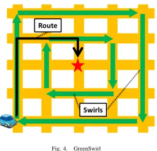
A swirl is a single loop of the multiple GreenWaves formed by the GreenSwirl TSC. Vehicles can run at the legal speed limit on a swirl without stopping unless there is traffic congestion. Many swirls of different sizes are formed at the same time. Multiple swirls can be utilized for a single route (Fig. 4).
Fig. 4. GreenSwirl
1) GreenSwirl: The details of forming swirls are shown in
the following.
Forming swirls: Swirls are manually designed according to the road network and traffic pattern. For example, Beijing has three loop roads in its center, and traffic gets heavy on these roads. The design concept of these loop roads is close to that of GreenSwirl. Fig. 5 shows an example how swirls could be formed in Beijing.
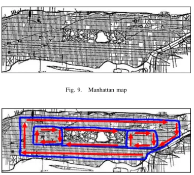
On the other hand, Manhattan has a park at its center, and there are many one-way streets. The traffic is prone to concentrate on the straight arterial streets, and we can form swirls to disperse this traffic (Fig.6).
Fig. 5. Forming swirls at Beijing
Fig. 6. Forming swirls at Manhattan
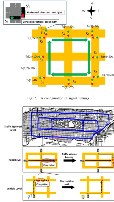
Configuring the timing of traffic signals: Fig. 7 shows an example of a configuration of signal timings. In this example, the first traffic signal is set as a green light; the time each vehicle takes to pass through a road segment is 10 sec. The signal timings must be carefully adjusted for the intersections where some vehicles on a swirl take a right or left turn. For example, suppose that the green period starts at 20 sec. for the north direction at S3. In this case, the vehicles can run directly
north or turn right without stopping at S3. At this time, S3′
(going east) is red. With GreenWave, the timing for S4 is set according to the distance from S3′, and this will stop the car that took a right turn at S3. With GreenSwirl, the timing for
S4is set according to the timing of S3 instead of S3′, and thus
the car on the swirl can pass through S4 without stopping.
2) GreenDrive: In order to reduce traffic congestion formed
by uneven traffic, a DRG for dissipating traffic is needed. The GreenDrive DRG estimates the travel time of each road segment and guides the vehicles in order to minimize the total travel time of the cars moving in the whole city. It utilizes previous traffic data and calculates the running time of a particular route by taking account of the number of right and left turns. GreenDrive guides the vehicles to the swirls so that the traffic is dispersed and the travel time of each car is reduced. Routes for vehicles are calculated at three levels (Fig. 8).
Road network level: The traffic at the city center is dispersed towards the swirls so that traffic congestion at the city center
Fig. 7. A configuration of signal timings
Fig. 8. GreenDrive
is reduced.
Road level: Although the traffic capacity of swirls is greater than that of other roads, swirls can get congested if the amount of traffic exceeds their capacity. With GreenDrive, the central server analyzes the travel time of each road segment collected by the sensors, and optimizes the traffic through route guidance given by navigation systems.
Vehicle level: The navigation system finds the route with the minimum travel time. The central server broadcasts the estimated travel time of each road segment, and the navigation system calculates the time to reach the destination along each of candidate routes. Then, the system guides the driver along the best route.
Green-Drive, these two methods differ in the following points. In order to balance the traffic, DUA determines the route for each vehicle by adjusting the selection probabilities of candidate routes. On the other hand, GreenDrive adjusts the estimated time to pass through each segment, and then the route for each vehicle is determined by finding the route that minimizes the total travel time to the destination.
Algorithm for GreenDrive
In order to deal with the fluctuation and concentration of traffic, GreenDrive adjusts the estimated time for passing through each segment and finds the optimal traffic pattern. It first calculates the estimated time from the legal speed limit of each road segment and gradually changes this estimate according to the real traffic, and thus reaches the optimal traffic. The pseudo code of the algorithm for finding the optimal routes for all cars is shown below.
Algorithm 1 GreenDrive Algorithm
1: Input P : Depature places and destinations for all vehicles 2: Input S ={s0, ..., sk}: Set of all road segments
3: Input E0={e0,s0, ..., e0,sk}: Set of initial estimated travel time
for all road segments
4: Parameter N : Number of iteration
5: Parameter z: Number of road segments to update 6: Parameter γ: Smoothing factor
7:
8: R = RBEST = k ShortestT imeRoute(P, S, E0);
9: // R: Travel routes for all vehicles
10: // RBEST: The best routes for all vehicles so far
11: for n = 1→ N do
12: M = SU M O Simulate(R, S);
13: // M = {ms0, ..., msk}: Observed travel time for all road
segments
14: for each s∈ S do
15: if s∈ the top z congested road segments in M then 16: en,s= γen−1,s+ (1− γ)ms; 17: else 18: en,s= en−1,s; 19: end if 20: end for 21: En={en,s0, ..., en,sk}; 22: R = k ShortestT imeRoute(P, S, En);
23: if total travel time for R is shorter than RBEST then
24: RBEST = R;
25: end if 26: end for 27: return RBEST;
The inputs for this algorithm are the places of departure and the destinations of all vehicles, the initial estimated travel time for all road segments and the set of all road segments. The initial estimation of travel time for a road segment can be calculated from its length and the legal speed limit. The output of the algorithm is the best combination of routes for the all vehicles which can minimize the average travel time.
Line 8: Based on the initial estimation of the travel time for each road segment, the tentative travelling route for each vehicle is determined. These routes are found by functionk ShortestP athRoute(P, S, E), which executes the k-shortest time paths algorithm which is described later.
Line 11–26: The searches for the best traffic are iterated N times.
Line 12: The traffic simulator SUMO is executed with the tentative travelling route for each car, and M is substituted for the observed travel time at each road segment.
Line 14–20: Based on the result of the simulation, the top z congested road segments are selected, and the estimated travel time for these road segments are updated to reflect the observed travel time. Based on the exponential moving average, we use Equation (1) to update the estimation. The coefficient γ represents a smoothing factor, and the default value for γ is 0.99. We need to make γ closer to 1 if the number of vehicles is high, in order to make the transition of the values smoother. As for the non-congested road segments, the estimation is not updated.
en,s= γen−1,s+ (1− γ)ms (1) Line 21–25 : Based on the updated estimation, the tentative travelling routes are updated by executing the k-shortest time paths algorithm. Then the total travel time for the all vehicles is calculated, and RBEST is updated if necessary.
k-shortest time paths algorithm
The k-shortest time paths algorithm finds the top k-shortest time paths for each vehicle taking account for the time for making right or left turns from the travel time at each road segment. In order to distribute the entire traffic, it chooses one route from the top k-shortest time paths at random.
IV. EVALUATION
In this section, we show the results of our evaluation-by-simulation, which uses the real road network of Manhattan in New York.
A. Simulation Settings
We used Simulation of Urban Mobility (SUMO) simulator [20], [21], [22] for our simulation-based study. We used the road network of Manhattan, which is shown in Fig. 9. The data for road network is taken from OpenStreetMap [23]. The size of the road network is 4km× 20km. The main streets in this network are two-way with two lanes for each direction. There are also many one-way streets. We set the maximum speed to
60km/h. The maximum density of vehicles was limited to 33
cars/km due to limitations of the simulator. The number of vehicles was determined for four cases: 5000, 10000, 15000 and 20000. The positions of departure and arrival for each vehicle were set at random. We generated 30 cars each second, and the simulation was executed for 50000 seconds.
Proposed method: For the proposed method, we configured the blue roads as GreenSwirl roads shown in in Fig. 10. The inner GreenSwirl roads are main roads with a high capacity. We set k = 1 or 3 and the parameter z to be 25. We changed the number of vehicles and γ in the following 4 cases (number of cars; γ): (5000, 0.99), (10000, 0.999), (15000, 0.9995) and
(20000, 0.9999). The number of iterations N for GreenDrive
Fig. 9. Manhattan map
Fig. 10. Construction of GreenSwirl road
B. Methods compared
The proposed method is a combination of GreenSwirl TSC and GreenDrive DRG. Therefore, we compared GreenSwirl with other TSC methods and GreenDrive with other DRG methods.
The methods we compared for TSC are the following: • Synchronized: This is the default signal control method
implemented in SUMO. In this method, all traffic signals change at the same time.
• GreenWave: GreenWave TSC is used for the main streets with a high traffic capacity. Fig.11 shows the streets with GreenWave TSC. For other streets, the default synchro-nized method is used.
Fig. 11. Construction of GreenWave road
The methods we compared for DRG are the following: • Shortest-path: Each of the vehicles is guided along the
shortest path between the source and the destination. • DUA: Vehicles are guided by the DUA algorithm, which
is described in Section II. The evaluation was done by executing 1000 iterations of the DUA algorithm. Note that, whatever the method, it is not realistic to assume that navigation methods have a 100% rate of adoption. So
we tested different adoption rates for GreenDrive in our simulation, where we determined that, when the adoption rate is below 100%, the vehicles without the navigation method travel along the shortest path.
It is also unusual to assume that all the streets would be equipped with sensors for detecting traffic. So we compared the methods using different ratios of streets from which traffic data are available. We used the ratios 30%, 70% and 100%. In the case of 30% availability, we also added another case, where 1% of vehicles report back their positional information to the central server via cellular communication. This gives the following 4 cases:
• Sensor30%: Traffic information can be obtained from 30% of the streets.
• Sensor30%+Feedback1%: Traffic information can be obtained from 30% of the streets, and 1% of the all vehicles report back their positional information. • Sensor70%: Traffic information can be obtained from
70% of the streets.
• Sensor100%: Traffic information can be obtained from all streets.
C. Results of Simulation
Results of k-shortest time paths method
Fig. 12 shows the results with the k-shortest-time paths method combined with the GreenSwirl TSC. Note that the travel time increases as the value of k increases. This is an unexpected result, and the reason is that, since Manhattan has a lot of one-way streets, the second best route is usually far worse than the best route. Based on this result, we abandoned the k-shortest time paths method and we only used the shortest time path method (k=1) in our subsequent evaluation.
Fig. 12. Travel time with k-shortest time paths method Comparison between TSC methods
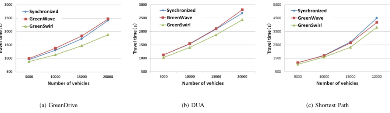
Fig. 13 shows the average travel time of vehicles comparing TSC methods. We compared the three TSC methods which use the three DRG methods. For the all combinations, the average travel time of the vehicles with GreenSwirl was the shortest. The reason that the synchronized TSC performed badly is that
vehicles are stopped frequently by randomly encountering red traffic signals. The shortest-path method was often the worst, since it does not provide alternative routes. The GreenWave TSC showed relatively good performance, and it was particu-larly good when combined with the GreenDrive or the DUA. In this case, however, the smaller streets close to the main streets are prone to heavy traffic, and some vehicles are guided along longer, time-consuming detour routes for dispersing traffic. As a result, GreenSwirl was better than GreenWave in the overall performance. The GreenSwirl method succeeded in dispersing traffic towards the peripheral of the city by creating multiple swirls throughout the city. Congestion was unlikely at any place with combinations of GreenSwirl and any of the DRG.
Results of route guidance methods
Fig. 14 shows how each DRG method reduces the average travel time. We compared the three DRG methods: (1) the shortest path method and (2) the DUA methods (both with a 100% adoption rate) and (3) the GreenDrive (in each of the cases of a 100%, 75%, 50%, and 25% adoption rate). We combined each of the TSC methods with these three DRG methods. The results show that the performance of the shortest-path method is poor, and this is because it does not disperse the traffic. With GreenSwirl, the performance with the DUA (100% adoption rate) was close to the performance with GreenDrive (50% adoption rate), but the GreenDrive performed better in the case of both 75% and 100% adoption rates. This is because the DUA does not focus on optimizing the individual route for each vehicle.
How the ratio of speed-detecting sensors to road segments affects the performance of the proposed method
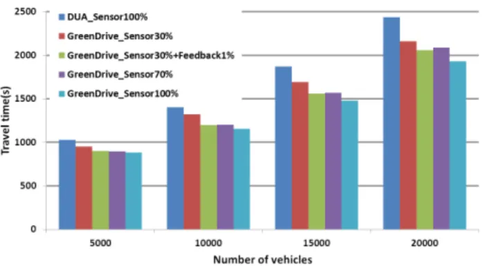
Fig. 15. The results for evaluating the proposed method with the different ratios of the road segments with speed-detecting sensors
We estimate that the actual installation rate of the traffic sensors on street segments is around 30%. Some models of the car navigation systems have functions for sending back traffic data to the server via cellular communication, and companies like Toyota, Nissan and Honda receive traffic data feedback from around 1% of all vehicles. We now evaluate the case in which 30% of streets have sensors installed for obtaining
traffic data and traffic data feedback is available from 1% of the vehicles.
Fig. 15 shows the results of comparing GreenDrive, un-der various conditions, and the DUA method–using the GreenSwirl TSC in both cases. We compared 5 cases (cases 1-4 here using GreenDrive): (1) 30% of streets with sensors installed; (2) 30% of streets with sensors installed, plus 1% of cars providing traffic data feedback; (3) 70% of streets with sensors installed; (4) 100% of streets with sensors installed; (5) the DUA method, for which the simulation used only 100% of streets with sensors installed–due to limitations of the SUMO simulator.
When the number of vehicles is 5000, there is almost no congestion and thus there is no need to adjust the traffic pat-tern. The GreenDrive method with 30% of sensor installation showed the worst results due to scarcity of data. However, when the 1% feedback data are added, GreenDrive showed satisfactory results.
When the number of vehicles is 10000, this “ medium ” amount of traffic with the DUA method showed the worst results. since DUA does not adjust the overall traffic.
When the number of vehicles is 15000, a considerable amount of traffic, the results were similar to those with 10000. We see that the results with the GreenDrive using 30% sensor installation + 1% feedback data are close to GreenDrive with 70% sensor installation. This is because the available feedback data increase as the number of vehicles increases.
When the number of vehicles is 20000, the traffic is even heavier, but the results resemble those with 10000 or 15000 vehicles. GreenDrive with 30% sensor installation + 1% feedback data is now better than GreenDrive with 70% sensor installation and is close to the method with 100% sensor installation. These results show that even a small amount of traffic feedback can have a significant and favorable impact on reducing traffic congestion.
V. CONCLUSION
In this paper, we proposed a traffic signal control method, GreenSwirl, and a route guidance method, GreenDrive. We conducted a simulation-based study with the SUMO traffic simulator and confirmed that GreenSwirl can reduce average travel time by 10-20% compared to GreenWave, and that GreenDrive can reduce the travel time by 10-60% compared to the existing methods. In the future, we will evaluate the performance of our methods in other cities such as Beijing (China), San Franciso (Bay area). We will also evaluate the scenarios in morning and evening rush-hour traffic.
REFERENCES
[1] J. Wang, M. Hu, C. Xu, G. Christakos and Y. Zhao, “ Estimation of citywide air pollution in Beijing, ”in PLoS ONE, 8(1): e53400. doi:10.1371/journal.pone.0053400, Jan. 2013.
[2] En. JieJing. ORG, “ Beijing congested road PM 2.5 exceeded twice the number of vehicles to be controlled,”http://en.jiejing.org/view-2411. html, Jul. 31, 2013 [Sep. 1, 2014].
[3] X. Li, F. Zeng, G. Chen and W. Ding,“ Design of a multi-route optimal simulation system for urban traffic controls, ”in Computer Engineering & Science, vol.10, pp.126-130, Oct. 2010.
(a) GreenDrive (b) DUA (c) Shortest Path
Fig. 13. Comparison of travel time using Synchronized,GreenWave,and GreenSwirl with different DRGs
(a) GreenSwirl (adoption rate of GreenDrive is 100%, 75%, 50%, 25%)
(b) GreenWave (adoption rate for all methods is 100%)
(c) Synchronized (adoption rate for all meth-ods is 100%)
Fig. 14. Comparison of travel time using Random,Dijkstra,DUA,and GreenDrive with different TSCs
[4] S. Tsugawa, M. Aoki, A. Hosaka and K. Seki,“A survey of present ivhs activities in Japan, ”in Control Engineering Practice, Vol.5, pp.1591-1597, Nov. 1997.
[5] M. Behrisch, D. Krajzewicz, P. Wagner, and Yun-Pang Wang,“Compari-son of Methods for Increasing the Performance of a DUA Computation,” in Proc. of DTA2008 International Symposium on Dynamic Traffic Assignment, No. EPFL-CONF-154987, Jun. 2008.
[6] D. Krajzewicz, M. Behrisch and Y. Wang, “ Comparing performance and quality of traffic assignment techniques for microscopic road traffic simulations,”in Proc. of DTA2008 International Symposium on Dynamic Traffic Assignment, No. EPFL-CONF-154987, Jun. 2008.
[7] E. Martins and M. Pascoal, “ A new implementation of yen’s ranking loop less paths algorithm, ”in Quarterly Journal of the Belgian, French and Italian Operations Research Societies, Vol.1,Issue 2, pp.121-133, Jun. 2003.
[8] J. Hershberger, M. Maxel and S. Suri, “ Finding the k shortest simple paths: A new algorithm and its implementation, ”in ACM Transactions on Algorithms (TALG), Vol.3, Issue 4, pp.26-31, Nov. 2007.
[9] A. Warberg, J. Larsen and R. Jrgensen,“ Green Wave Traffic Optimiza-tion - A Survey, ”in Informatics and Mathematical Modeling, 2008. [10] M. Sasaki, T. Nagatani, “ Transition and saturation of traffic flow
controlled by traffic lights, ”in Physica A: Statistical Mechanics and its Applications, Vol.325, Issues 3-4, pp.531-546, Jul. 2003.
[11] BBC News,“ Drivers catch green lights ‘wave’, ”http://news.bbc.co.uk/ 2/hi/uk news/7998182.stm, Apr. 14, 2009 [Sep. 1, 2014].
[12] T. Ikeda, E. Kitagawa and E. Morimatsu, “ Environmental evaluation of non-stop driving assistance service by high-spatiotemporal resolution traffic simulator, ”in 17th ITS World Congress, 2010.
[13] R. Junges, and A.L. Bazzan, “ Evaluating the performance of DCOP algorithms in a real world, dynamic problem, ”in Proc. of the 7th International Joint Conference, Vol.2, pp.599-606, 2008.
[14] G. Shen and W. Xu,“Study on traffic trunk dynamic two-direction green wave control technique,”in Journal of Zhejiang University (Engineering Science), Vol.42, pp.1625-1630, 2008.
[15] H. Taale, “ Comparing methods to optimise vehicle actuated signal control, ”inRoad Transport Information and Control, pp.114-119, 2002. [16] D. Robertson and R. Bretherton,“Optimizing networks of traffic signals in real time - the scoot method, ”in IEEE Transactions on Vehicular Technology, Vol.40, No.1, 1991.
[17] V. Gradinescu, C. Gorgorin, R. Diaconescu, V. Cristea and L. Iftode,
“ Adaptive traffic lights using car-to-car communication ”, in Proc. of
IEEE 65th Vehicular Technology Conference (VTC 2007 Spring), pp.21-25, Apr. 2007.
[18] eCoMove (2009). Annex I - “ Description of Work ” of the eCoMove project, Project reference FP7-ICT-2009-4.
[19] Paul Mathias, Jonas L¨ußmann, Claudia Santa, Jaap Vreeswijk and Matthias Mann, “ Traffic network simulation environment for the co-operative eCoMove system”. In 19 th Intelligent Transportation Systems World Congress, Vienna, Austria.
[20] M. Behrisch, L. Bieker, J. Erdmann and D. Krajzewicz, “ Sumo -simulation of urban mobility: An overview, ”in Proc. of The Third International Conference on Advances in System Simulation, pp.63-68, 2011.
[21] D. Krajzewicz, G. Hertkorn, C.Rossell and P. Wagner, “ Sumo (simu-lation of urban mobility), ”in Proc. of The 4th Middle East Symposium on Simulation and Modeling, pp.183-187, 2002.
[22] D. Krajzewicz, E. Brockfeld, J. Mikat, J. Ringel, C.Rossel, W. Tuch-scheerer, P. Wagner and R. Wosler,“ Simulation of modern traffic lights control systems using the open source traffic simulation sumo, ”in Proc. of The 3rd industrial simulation conference, Vol.2205, pp.299-302, 2005. [23] OpenStreetMap homepage, http://www.openstreetmap.org/, Aug. 9,