Phase-Modulation Fluorometer Using a Phase-Modulated Excitation Light Source

Phase-Modulation Fluorometer Using a Phase-Modulated Excitation Light Source

Takahiko Mizuno, Yasuhiro Mizutani, and Tetsuo Iwata*

Division of Energy System, Institute of Technology and Science, The University of Tokushima, 2-1 Minami-Jyosanjima, Tokushima 770-8506, Japan

* _{E-mail address: iwata@me.tokushima-u.ac.jp}

Abstract

We propose a phase-modulation fluorometer (PMF) with a light-emitting diode (LED) or a laser diode (LD) used as an excitation light source (ELS) that is driven in the phase-modulation (PM) mode. The PM-ELS generates many frequency sidebands that spread in the vicinity of carrier frequency fc with the interval of modulation frequency fm depending on the maximum phase deviation _{Δ . The scheme enables us to derive fluorescence lifetime φ} values of a multicomponent sample at one time. We show a typical numerical simulation result for explaining the principle of operation. To demonstrate the effectiveness of the proposed PMF, we have measured fluorescence lifetimes of three kinds of inorganic fluorescent glasses and that of a mixture solution of 1 10−6

× M rhodamine 6G and 1×10−6M

coumarin 152 in ethanol with a volume ratio of 1 :1.

Keywords: phase-modulation fluorometer, phase-modulated light source, fluorescence lifetime, spectroscopic techniques, instrumentation

1. Introduction

In analytical chemistry, biochemistry, and organic- and inorganic-material science, fluorescence lifetime measurements play an important role in analyses for distinguishing samples. On the basis of fluorescence lifetime values, we are often able to distinguish between two fluorescent samples whose spectral shapes are similar to each other and which would otherwise be indistinguishable.

Measurement methods for obtaining fluorescence lifetime values are divided into two categories: time-domain (TD) methods and frequency-domain (FD) methods1). In the TD method, we measure the impulse response of the fluorescence sample after pulsed excitation. In this case, we are able to obtain a fluorescence decay waveform directly and to measure weak fluorescence with precision by adopting a time-correlated single-photon-counting (TC-SPC) technique. This is the reason why the TC-SPC method has been utilized commonly. However, safety and damage considerations for the sample are required. Consideration to avoid the nonlinear optical effect is also required. On the other hand, the FD method is the measurement of the steady-state response of the sample for sinusoidally modulated excitation. Therefore, the FD method seems promising for use with biological samples. However, we have to use plural modulation frequencies to measure a multicomponent fluorescent sample. To solve this problem, a mode-locked laser with a high-repetition frequency has been used as an excitation light source (ELS); phase shifts of many harmonics of the fundamental repetition frequency are utilized for obtaining fluorescence lifetime values. Such a system works quite well for analytical purposes in the laboratory. However, the use of the mode-locked laser system results in some complications in constructing the total measurement system, troublesome adjustment and maintenance, large size, and high cost. In addition, flexibility for selecting the optimal excitation wavelength for the absorption band of the sample is restricted.

diodes (LD) that have recently become available have alleviated the difficulties. Among the many FD instruments developed so far, the conventional PMF equipped with the LED (or LD) as the ELS is easy to construct and simple in operation2-6), where the conventional PMF means the traditional one that uses a single or a few modulation frequencies at most. Depending on kind of the fluorescent sample, the LED (or LD) can be replaced easily with another one so that its emission wavelength matches the absorption band of the sample. Therefore, the conventional PMF is still useful for the purpose of screening biological samples. However, two problems arise in practical application: (i) the use of PMF is limited to fluorescent samples whose quantum efficiencies are moderately high, and (ii) the fluorescence decay curve should be expressed by a single-exponential function. The former problem might be alleviated by using a photon-counting PMF7). For the latter problem, the use of a PMF with plural modulation frequencies has been proposed8-22)_{. We also have proposed a} Fourier-transform (FT)-PMF23,24) and a frequency-multiplexed (FMX)-PMF25) incorporated with the UV or the blue LED. Although the two PMF’s work well, there still remains a problem in preparing the excitation waveform peculiar to each PMF, which is somewhat cumbersome: we need a frequency-chirped waveform for the FT-PMF and a frequency-multiplexed and phase-randomized one for the FMX-PMF. Such a general-purpose waveform generator is difficult to prepare in a practical analytical situation. Furthermore, for the case of the FMX-PMF, the number of modulation frequencies and that of data points were limited to less than 10 and 3,000 at most, respectively, because of the tremendous computation-time problem due to the autoregressive-model-based data-analysis technique. A simple PMF that is easy to construct is required.

In the present paper, although the final goal and the fundamental principle for deriving fluorescence lifetime values are the same as described in the previous one, we propose an

alternative technique and concept of PMF for solving the problem: the use of a phase-modulated excitation light source (PM-ELS). With the PM-ELS, we are able to obtain many sidebands that spread over at the upper and the lower side of carrier frequency fc with the interval of modulation frequency fm. In the present paper, for the sake of simplicity, we use an arbitrary waveform generator and a digital oscilloscope for generating and recording the PM waveform, respectively, as before.25) However, we can easily replace them anytime with two commercially available phase-locked-loop integrated circuits (PLL-IC). To our knowledge, no such idea or instrumental technique has yet been reported. To demonstrate the performance of the proposed PMF, we have measured fluorescence lifetime values of three kinds of inorganic fluorescent glasses and that of a mixture solution of 1_×10−6_{M rhodamine}

6G and 1_×10−6_{M coumarin 152 in ethanol with a volume ratio of 1 :1.}

2. Principle of PMF with PM-ELS

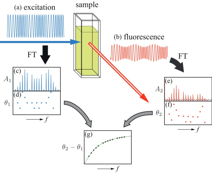
Figure 1 shows a conceptual diagram that illustrares the principle of PMF with PM-ELS. The PM excitation waveform (a) as a function of time t is given by

(

)

{

f t f t

}

A t

e( )= cos2

π

_c +Δ

φ

cos2

π

_m , (1)

where fc is the carrier frequency, fm is the modulation frequency, and Δ is the maximum φ phase deviation. The fluorescence waveform (b) is given by the convolution of the excitation wave (a) with the fluorescence decay wave that would be obtainable from the impulse excitation. Waveforms (c) and (d) are the modulus A1(f) and the phase spectrum

θ

1(f), respectively, which are obtainable by Fourier transform of the excitation waveform (a). Similarly, waveforms (e) and (f) are the modulus A2(f)and the phase

θ

2(f) spectrum, respectively, obtainable from the fluorescence waveform (b). The two waveforms (c) and (e) have many sidebands around the carrier frequency fc with the interval of fm. The number and

magnitudes of the sidebands depend on _{Δ . The horizontal dotted line depicted in (e) [and φ} (c)] indicates a threshold level, which is used for calculating the discrete phase-difference spectrum

θ

(f)=

θ

1(f)−

θ

2(f) shown in (g). When calculating θ( f) from (d) and (f),

uninformative phase components are discarded: that is, the phase spectral components whose corresponding modulus spectra below the threshold level in magnitude are made to be zero. This is because such components are embedded in noise in a practical situation. From θ( f), we can derive a fluorescence lifetime value (or values) by the conventional procedure in PMF1)_{. In this manner, measurements at plural modulation frequencies can be carried out at} one time.

We can carry out precise measurements by chooing the optimal PM parameters of fc, fm, and

φ

Δ for a given or an unknown fluorescence lifetime value of τ . From the equation

θ τ

π tan

2 f = , we can derive the following relation:

θ θ τ τ 2 sin 2Δ = Δ _{. (2)}

The optimal modulation frequency that gives the minimum value of Δτ/τ is fopt =1/2πτ

and then θ =π /4. We therefore should determine f so as to be equal toc f , taking into opt

account the other PM parameters. Although we should set the value of Δ to be large so as φ

to cover a wide frequency range, a large value of Δ results in small magnitude in the φ

modulus spectrum. We therefore empirically set the threshold level as 10 % against the peak value, although the level should be changed depending on τ , noise level, and the number of accumulations of waveforms. For the 10 %-thereshold level, we set Δ_φ=2_π to generate around ten sideband spectral lines and set f_m= fc/ 10 to cover the frequency range of around 10 f .

In principle, the overall noise-proof capability of the proposed PMF is the same as that of the conventional one from the viewpoint of signal-gathering efficiency. However, the proposed PMF enables us to use plural modulation frequencies at one time. Extending the above procedure to a multicomponent sample is straightforward1,16). Even for the single-component, the proposed PMF is useful for readily confirming whether it actually consists of a single component.

3. Numerical Simulation

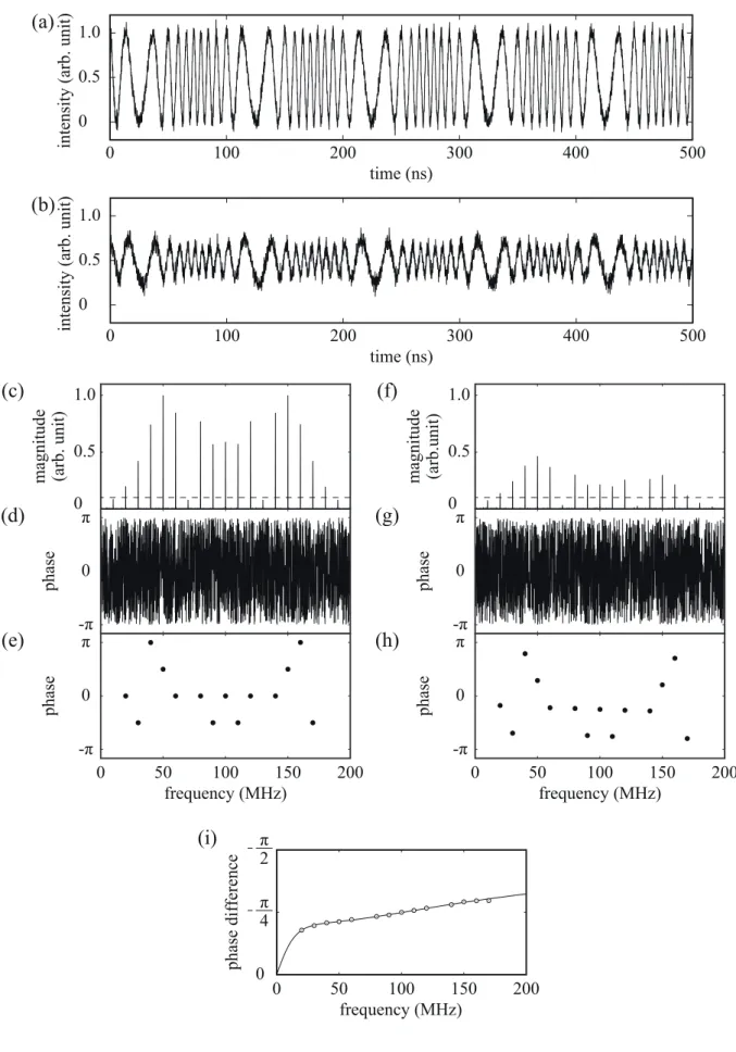
In order to demonstrate that the proposed PMF works well for the multicomponent sample in a situation with noise, we carried out a numerical simulation, in which two different series of artifitial noise were added to the excitation and the fluorescence waveform independently. Figure 2(a) shows the PM excitation waveform, where Δ_φ =2_π, fc= 100 MHz, and fm = 10 MHz. We set the sampling frequency fs to be 25 GHz (data interval; Δt= 40 ps) and the number of total data points N = 10,000. Figure 2(b) shows the fluorescence waveform, where we assumed that the fluorescence decay waveform was expressed as the sum of two exponentials: f(t)=a₁exp

₍

−t/

τ

₁

₎

+a₂exp

₍

−t/

τ

₂

₎

, where

τ

1=10.0 ns,

τ

2 =1.0 ns, and

=

1

2/ a

a 5.0. For the excitation and the fluorescence waveform, we superimposed =

σ 5 %-Gaussian-distributed noise against the peak-to-peak value, where σ is a standard deviation of Gaussian noise. Figures 2(c) and 2(d) show Fourier transforms of (a): (c) is a modulus spectrum and (d) a phase spectrum. Similarly, Figs. 2(f) and 2(g) show Fourier transforms of (b): (f) is a modulus spectrum and (g) a phase spectrum. Figure 2(e) shows a plot of phase values versus modulation frequency, which was extracted from (d) using the 10 % threshold level depicted in (c). Similarly, Fig. 2(h) shows a plot of phase values versus modulation frequency, which is obtained from (g) using (f). Figure 2(i) shows a phase

difference spectrum θ( f) calculated from (e) and (h). The solid line shows the theoretically calculated curve for the true values of

τ

₁=10.0 ns,

τ

₂=1.0 ns, and a₂/ a₁=5.0. In this

fashion, we carried out thirty independent numerical trials to evaluate the influence of noise on the assumed true values. The estimated values were

τ

ˆ₁=9.9±0.1 ns,

τ

ˆ₂ =1.0±0.1 ns, and

=

1

2/ a

a 4.9±0.1 ns. In spite of adding σ =5 %-Gaussian noise to both the excitation and the fluorescence waveform independently, the proposed scheme worked well.

4. Experimental Setup

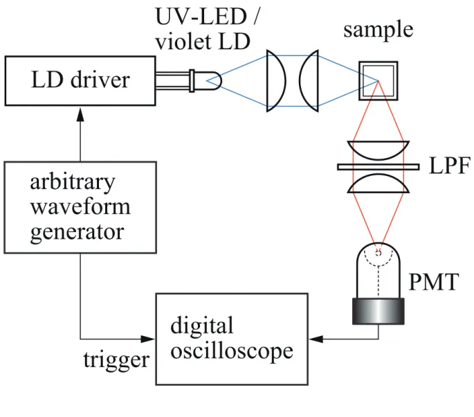
Figure 3 shows a schematic diagram of the proposed PMF with PM-ELS. In order to demonstrate the performance of the PMF, we carried out two basic measurements. The first one was the measurement of fluorescence lifetime values of three kinds of fluorescent glasses that are commercially available: Lumilass B, Lumilass G9, and Lumilass R7 (Sumita Optical Glass) with peak absorption and emission wavelengths of 353 nm and 413 nm, 315 nm and 543 nm, and 393 nm and 613 nm, respectively. Here, we used a UV LED (NSHU590E, Nichia) as the PM-ELS, the peak emission wavelength of which was 365 nm. The UV LED was driven with a 15 mA dc bias current, and a 20 mApp PM signal obtained from an arbitrary waveform generator (AWG 520, Tektronix) was superimposed on the dc bias. Average light power on the sample point was about 10 nW. We inserted a low-pass filter (LPF) in the emission side: SCF-50S-42L (–3dB cutoff wavelength λ_c= 420 nm, Sigma Koki) for the case of Lumilass B, SCF-50S-48Y (λc= 480 nm) for that of Lumilass G9, and SCF-50S-58O

(λc= 580 nm) for that of Lumilass R7. When obtaining the reference waveform, we replaced

each sample by a diffusion plate that had no wavelength dependence in reflection. The output signal obtained from a photomultiplier tube (PMT; 7400U, Hamamatsu Photonics) was fed

into a digital oscilloscope (TDS5054, Tektronix), in which an accumulation procedure was carried out 1,000 times for N = 5,000. For demonstrative purposes, we used two pairs of PM parameters (fc, fm) for the fixed value of Δφ=2π so that two decades of the frequency bandwidth was covered: (i) (fc, fm) = (50, 5.0 kHz) and (ii) (500, 50 kHz) for the case of Lumilass B, (i) (500, 50 Hz) and (ii) (5.0 kHz, 500 Hz) for that of Lumilass G9, and (i) (500, 50 Hz) and (ii) (5.0 kHz, 500 Hz) for that of Lumilass R7.

The second measurement is that of fluorescence lifetime values of 1_×10−6_{M rhodamine}

6G in ethanol, _1×10−6_{M coumarin 152 in ethanol, and a mixture of the two solution a volume}

ratio of 1 :1. The peak wavelength of absorption and that of emission of rhodamine 6G were 531 and 553 nm, respectively. Those of coumarin 152 were 400 and 505 nm, respectively. For these measurements, we used a violet LD (NDV4313, Nichia) as the PM-ELS, the emission wavelength of which was 405 nm. The violet LD was driven with a 70 mA bias current and a 40 mApp PM signal was superimposed on it. The average power on the sample point was about 65 µW. The experimental procedure was the same as above, except that the number of accumulations and that of sampling points were increased from 1,000 to 10,000 and 5,000 to 100,000, respectively. We inserted LPF on the emission side: SCF-50S-48L (λc= 480 nm) for

the case of rhodamine 6G and SCF-50S-42L (λc= 420 nm) for that of coumarin 152 or the

mixture solution. In these measurements, we again used two pairs of PM parameters for the fixed value of Δ_φ=2_π: (i) (fc, fm) = (20, 2.0 MHz) and (ii) (100, 10 MHz).

5. Results and Discussion

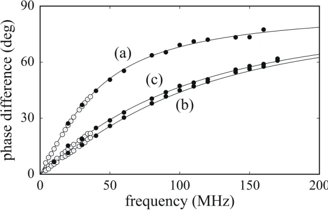
Figures 4(a)-4(c) show plots of phase difference versus frequency, which were obtained from the three fluorescent glasses: (a) Lumilass B, (b) Lumilass G9, and (c) Lumilass R7. We

plotted modulation ratio spectra as well as phase difference spectra for reference purposes. In each figure, the solid line shows the theoretically calculated curve. Plots of white circles and black circles represent data points obtained from the PM parameters (i) and (ii), respectively, as described in the experimental section. Concerning Lumilass B and Lumilass R7, we found that their fluorescence decays could be approximated by a single-exponential function with

=

τˆ 792±0.1 ns and τˆ=2.15±0.01 ms, respectively. For Lumilass G7, however, we found that

the decay could not be approximated by a single-exponential one. As shown in the figure, the decay should be expressed as the sum of two exponentials: aˆ₁exp(−t/

τ

ˆ₁)+aˆ₂exp(−t/

τ

ˆ₂),

where

τ

ˆ₁₌2.31±0.01 ms,

τ

ˆ2 =35.5±0.1 ns, and aˆ a2/ ˆ1=850±10. At present, we have no means to confirm whether the estimated fluorescence lifetime values are true because no reliable information on compositions of the fluorescence glasses is available from the manufacturer’s data sheet26). However, our measurements with different PM parameter settings support the estimated results.

Figure 5 shows plots of phase difference versus frequency for (a) _1×10−6_{M rhodamine 6G}

in ethanol, (b) 1 10−6

× M coumarin 152 in ethanol, and (c) the mixture solution. Again, solid

lines show theoretically fitted curves: estimated values are (a) τˆ=4.0±0.1 ns, (b) τˆ=1.6±0.1

ns, and (c)

τ

ˆ₁=4.0±0.1 ns,

τ

ˆ₂ =1.6±0.1 ns, and aˆ a2/ ˆ1=11±0.5. The lifetime value of rhodamine 6G and that of coumarin 152 agree well with literature values27,28). For the mixture solution, the ratio of aˆ₂

τ

ˆ₂/aˆ₁

τ

ˆ_1≅4.4 is almost equal to that of the total fluorescence intensities

of the two solutions separately measured using a fluorescence spectrometer (RF−5300PC, Shimadzu) with the excitation wavelength of 405 nm.

The measurement results shown above indicate that the proposed PMF is useful for estimating fluorescence lifetime values of a multicomponent sample as well as a

single-component one. Although we have proposed the use of PM-ELS in the present paper, we can also use a frequency-modulated (FM)-ELS for the same purpose. However, the PM-ELS might be somewhat easier to use than the FM-ELS. This is because we can determine the frequency bandwidth of the PM-ELS from only Δ independent of fφ m.

6. Conclusions

We have proposed a concept of a phase-modulation fluorometer (PMF) that incorporates a phase-modulated (PM) excitation light source (ELS). In the proposed PMF, frequency sidebands obtainable from the PM-ELS were used for estimating fluorescence lifetime values of a multicomponent fluorescent sample at one time. Even for a single-component sample, the proposed PMF is useful for confirming whether it actually consists of a single-component. Although we used an arbitrary waveform generator and a digital oscilloscope for obtaining the PM excitation waveform and recording the fluorescence waveform, respectively, we could use two commercially available PLL-ICs for modulation and demodulation purposes. Such a modification and the use of an amplitude limiter might improve the carrier-to-noise ratio of the PM waveform further, which is a common technique used in FM communication. The proposed PMF is easy to construct and simple in operation and has the potential for use in the screening of fluorescent samples.

Acknowledgements

This work was supported by a Grant-in-Aid for Scientific Research (B) No.21300167 from Japan Society for the Promotion of Science (JSPS).

References

1) J. R. Lakowicz: Principle of Fluorescence Spectroscopy (Springer, New York, 2006) 3rd edition.

2) J. Sipior, G. M. Carter, J. R. Lakowicz, and G. Rao: Rev. Sci. Instrum. 68 (1997) 2666. 3) P. Harms, J. Sipior, N. Ram, G. M. Carter, and G. Rao: Rev. Sci. Instrum. 70 (1999)

1535.

4) T. Iwata, T. Kamada, and T. Araki: Opt. Rev. 7 (2000) 495. 5) H. Szmacinski and Q. Chang: Appl. Spectrosc. 54 (2000) 106. 6) P. Herman and J. Vecer: Ann. N. Y. Acad. Sci. 1130 (2008) 56. 7) T. Iwata, A. Hori, and T. Kamada: Opt. Rev. 8 (2001) 326.

8) R. D. Spencer and G. Weber: Ann. N. Y. Acad. Sci. 158 (1969) 361.

9) H. Merkelo, S. R. Hartman, T. Mar, and G. S. Singhal Govindjee: Science 164 (1969) 301.

10) M. J. Wirth and S. Chou: Appl. Spectrosc. 42 (1988) 483.

11) F. V. Bright, C. A. Monig, and G. M. Hieftje: Anal. Chem. 58 (1986) 3139. 12) F. V. Bright, C. A. Monig, and G. M. Hieftje: Appl. Opt. 26 (1987) 3526. 13) F. V. Bright, C. A. Monig, and G. M. Hieftje: Appl. Spectrosc. 42 (1988) 272. 14) M. Hauser and G. Heidt: Rev. Sci. Instrum. 46 (1975) 470.

15) H. P. Haar and M. Hauser: Rev. Sci. Instrum. 49 (1978) 632.

16) G. Ide, Y. Engelborghs, and A. Persoons: Rev. Sci. Instrum. 54 (1983) 841. 17) E. Gratton and M. Limkeman: Biophys. J. 44 (1983) 315.

18) E. Gratton, M. Limkeman, J. R. Lakowicz, B. P. Maliwal, H. Cherek, and G. Laczko: Biophys. J. 46 (1984) 479.

(1984) 463.

20) B. A. Fedderson, D. W. Piston, and E. Gratton: Rev. Sci. Instrum. 60 (1989) 2929. 21) E. Gratton, D. M. Jameson, N. Rosato, and G. Weber: Rev. Sci. Instrum. 55 (1984) 486. 22) S. A. Vinogradov, M. A. Fernandez-Searra, B. W. Dugan, and D. F. Wilson: Rev. Sci.

Instrum. 72 (2001) 3396.

23) T. Iwata: Opt. Rev. 10 (2003) 31.

24) T. Iwata, H. Shibata, and T. Araki: Meas. Sci. Technol. 16 (2005) 2351. 25) T. Iwata, A. Muneshige, and T. Araki: Appl. Spectrosco. 61 (2007) 950. 26) http://www.sumita-opt.co.jp/en/functional/lumilass.pdf.

27) D. Magde, R. Wong, and P. G. Seybold: Photochem. Photobiol. 75 (2002) 327.

Figure Captions

Fig.1 Illustration of the principle of PMF with PM excitation light source.

Fig.2 Numerical simulation result for PMF with PM excitation light source. (a) PM excitation waveform e(t) with Δφ=2π, fc = 100 MHz, and fm = 10 MHz, where fs = 25 GHz and N = 10,000, (b) fluorescence waveform with

τ

₁=10.0 ns,

τ

₂ =1.0 ns,

and a₂/ a₁= 5.0. σ = 5 %-Gaussian-distributed noise was added on the two waveforms (a) and (b) independently. (c) and (d) are Fourier transforms of (a): (c) is a modulus spectrum and (d) is a phase spectrum. (f) and (g) are Fourier transforms of (b): (f) is a modulus spectrum and (g) is a phase spectrum. (e) and (h) are plots of phase values extracted from (d) and (g), respectively, using threshold levels shown in (c) and (f). (i) Phase difference spectrum, where solid line shows theoretically calculated values for

τ

1=10.0 ns,

τ

2 =1.0 ns, and a2/ a1=5.0.

Fig.3 Schematic diagram of the proposed PMF. For the measurements of fluorescent glasses, a 365 nm UV LED was used and for that of rhodamine 6G and coumarin 152, a 405 nm LD was used as the ELS.

Fig.4 Phase difference spectra for three kinds of fluorescent glasses: (a) Lumilass B, (b) Lumilass G9, and (c) Lumilass R7, where modulation ratios as well as phase differences are plotted for reference. In each plot, the solid line shows the theoretically calculated curve. White and black circles represent data points obtained from PM parameters (i) and (ii), respectively, as described in the experimental section.

Fig.5 Phase difference spectra: (a) _1×10−6_{M rhodamine 6G in ethanol, (b) 1×10}−6_M

coumarin 152 in ethanol, and (c) a mixture of the two solutions at a volume ratio of 1 : 1. In each plot, the solid line shows the theoretically calculated curve. White and black

Figure 1

sample

(a)

excitation

(b)

fluorescence

FT

FT

f

(g)

f

(c)

(d)

f

(e)

(f)

Figure 2

frequency (MHz) 0 50 100 150 200 ph as e d iff er en ce π 2 π 4 0 (i) in te ns ity (a rb . u ni t) time (ns) 1.0 0.5 0 0 100 200 300 400 (a) 500 (e) (d) magnitude (arb . u ni t) (c) phase phase π 0 -π frequency (MHz) 0 50 100 150 200 π 0 -π 1.0 0.5 0 (h) (g) (f) magnitude (arb.unit) frequency (MHz) 0 50 100 150 200 π 0 -π π 0 -π 1.0 0.5 0 phase phase (b) in te ns ity (a rb . u ni t) 1.0 0.5 0 time (ns) 0 100 200 300 400 500

Figure 3

LPF

sample

PMT

arbitrary

waveform

generator

digital

oscilloscope

LD driver

UV-LED /

violet LD

trigger

Figure 4

ph

as

e d

iff

er

en

ce

(d

eg

)

90 60 30 0 101 ₁₀2 ₁₀3 ₁₀4 ₁₀5 ₁₀6

frequency (Hz)

m

od

ul

at

io

n r

at

io

10-1 10-2 100

(a)

101 ₁₀2 ₁₀3 ₁₀4 ₁₀5 ₁₀6

(b)

(c)

101 ₁₀2 ₁₀3 ₁₀4 ₁₀5 ₁₀6

τ = 792 ns

τ

1

= 2.31 ms

τ

2

= 35.5 ns

a

2

/a

1

= 850

τ = 2.15 ms

10-1 10-2 100 10-1 10-2 100 90 60 30 0 90 60 30 0

m

od

ul

at

io

n r

at

io

m

od

ul

at

io

n r

at

io

ph

as

e d

iff

er

en

ce

(d

eg

)

ph

as

e d

iff

er

en

ce

(d

eg

)

frequency (Hz)

frequency (Hz)

Figure 5

frequency (MHz)

0

50

100

150

200

(a)

(b)

(c)

ph

as

e d

iff

er

en

ce

(d

eg

)

90

60

30

0