東京海洋大学学術機関リポジトリ　TUMSAT-OACIS

(1)

TUMSAT-OACIS Repository - Tokyo University of Marine Science and Technology (東京海洋大学)

Application and calibration of 2-dimensional

flowmodel for small tidal rivers with

insufficienthydrographic data in Vietnamese

Mekong Delta

学位名

博士(工学)

学位授与機関

東京海洋大学

学位授与年度

2020

学位授与番号

12614博甲第571号

URL

http://id.nii.ac.jp/1342/00001997/

(2)

Doctoral Dissertation

APPLICATION AND CALIBRATION

OF 2-DIMENSIONAL FLOW MODEL

FOR SMALL TIDAL RIVERS

WITH INSUFFICIENT HYDROGRAPHIC DATA

IN VIETNAMESE MEKONG DELTA

September 2020

Graduate School of Marine Science and Technology

Tokyo University of Marine Science and Technology

Doctoral Course of Applied Marine Environmental Studies

(3)

I

Abstract

In recent years, in the Vietnamese Mekong Delta (VMD) riverbank erosion and collapse have been excessively occurring in many rivers, especially in small rivers, and threatening people living near the riverbank not only their properties but also their future, even their lives. Erosion and collapse are predicted to increase significantly under the influence of tidal range, sea-level rise (SLR), and land subsidence. To confront with erosion and riverbank collapse, small rivers should be intensively studied together with large rivers as most recent studies. However, making research on small rivers in VMD, especially in modeling a depth-averaged two-dimensional (2-D) flow model, will be very difficult because of the lack of hydraulic data. The main objective of this study is to demonstrate how to apply and calibrate a 2-D flow model for small tidal rivers in the VMD with insufficient hydrodynamic data. Three primary problems on applying a 2-D flow model to these kinds of small tidal rivers are insufficient bathymetric data, insufficient data for setting up the open boundary conditions, and insufficient data for calibrating the parameters of the model. To solve these problems the following steps were proposed. First, two measurement campaigns were conducted to collect the field data, including depth samples along the river in zigzag distribution, total discharge at the upstream cross-section in 36 hours, daytime hourly water levels near the estuary of the study river (i.e. My Thanh River, Soc Trang Province, Vietnam). Next, a new searching method was proposed as an effective interpolation method to reproduce the river bathymetry with sparse zigzag depth data. Based on the estimated bathymetry, the method suggested by Takagi et al. (2019) was applied to a 2-D flow model for the study river with some modifications. Finally, the spatio-temporal velocity along the river recorded by Acoustic Doppler Current Profiler (ADCP) devices during the measurement campaigns was applied to re-calibrate and optimize the 2-D flow model. Four primary results were obtained at this research. First, a proposed searching method, named Curvilinear search, is the most suitable to apply with Inverse distance weighting (IDW), Ordinary Kriging (OK), and Radial Basis Functions (RBF) interpolation methods to estimate the bathymetry of the river using sparse zigzag data; and two regional interpolation methods (i.e. Curvilinear-IDW method for estimating the near riverbank areas combining with Curvilinear-RBF or Rectilinear-RBF method for estimating the middle river area, respectively) working effectively with this kind of data were also figured out. Second, it was

(4)

II

found that the Riemann boundary condition is very helpful in case of insufficient upstream discharge data but needs to be modified to be compatible with the 2-D flow model. Third, the suggested flow model was improved significantly after re-calibrating with spatio-temporal velocity, reviewing the primary tidal constituents, considering the upstream discharge, and downstream tributary. Particularly, Root-Mean-Square Error (RMSE) of estimated water levels near downstream, upstream, and depth-averaged velocity over upstream cross-section were declined by 50%, 9%, and 12%, respectively; the estimated spatio-temporal velocity was also optimized 16%. Finally, it was demonstrated that the proposed 2-D flow model can be easily applied to simulate the flow of a small tidal river in a long period by applying downstream tidal data and Riemann Boundary. This research will be helpful for other studies with similar field conditions in the future.

(5)

III

List of figures

Figure 1-1. The Vietnamese Mekong Delta. ...2 Figure 1-2. My Thanh River with field observation overall planning (a), and equipment setup (b). ...5 Figure 3-1. Convert ADCP data to depth samples... 17 Figure 3-2. Distribution of classified depth sample data: calculating data (a, b) and calibrating data (c, d); and histogram graphs of their depth (c, d, f). ... 18 Figure 3-3. Previous and proposed searching methods... 20 Figure 3-4. Flowchart of interpolation Matlab program. ... 23 Figure 3-5. The estimated depth of C-IDW and R-IDW interpolator at four areas marked from a1 to a4 in Figure 3.2, and extracted depth profiles of four selected cross-sections from CS-a1 to CS-a4 in these areas. In the case of CS-a2, its location is near Cross-section 3, so the estimated depths were extracted at the measured locations... 25 Figure 3-6. The regional MAEs of using interpolators calculated at near riverbank areas (a) and the middle area of the river (b), the red-dash boxes show the suitable interpolators in this region... 26 Figure 3-7. Error profiles of estimated depths by applied interpolators at four cross-sections, their locations are marked in Figure 3-2. ... 28 Figure 4-1. Tidal data analysis: observation and harmonic analysis (a); max, min, and average values (b); and mean sea-level and linear trend (c). ... 33 Figure 4-2. Field data measured on 28th and 29th August 2018. ... 34 Figure 4-3. The 2D flow model of My Thanh River: the study area (a), the structure of the extended Riemann boundary. ... 37 Figure 4-4. The simulation results of My Thanh River: Water levels at Station A (a), Station B (b), and depth-averaged velocities over the upstream cross-section (c). ... 39 Figure 4-5. The spatial distribution of velocity vectors near the upstream cross-section: applied Riemann boundary at the upstream (a), extended Riemann Boundary (b). ... 40 Figure 5-1. Distribution of velocity data measured by the ADCP device. ... 45 Figure 5-2. The yearly changing of amplitude and phase of the primary constituents of the tide at My Thanh and Tran De station. ... 47 Figure 5-3. The new 2-D flow model of My Thanh River. ... 48

(9)

VII

Figure 5-4. The algorithm to estimate the model result of the spatio-temporally depth-averaged velocity. ... 52 Figure 5-5. The measurement data and simulation results of Chapter 4’s model: Water level at Station A (a), the averaged velocity at upstream, and spatio-temporally depth-averaged velocity on 28th_{, 29}th_{August 2018. ... 54}

Figure 5-6. Measurement and estimated water level at Station A, Station B, and depth-averaged velocity at the upstream of Case 0 and Case 1, the negative velocity means that the water flows to the upstream-ward direction. ... 55 Figure 5-7. Errors of the estimated spatio-temporally depth-averaged velocity on 28th and 29th August 2018 of simulation Case 0 and Case 1. ... 56 Figure 5-8. Cumulative discharges at Riemann-BC1 of simulation Case 1, Case 2, and Case 3. ... 57 Figure 5-9. Measurement and estimated depth-averaged velocity at the upstream of Case 1, Case 2, and Case 3. ... 58 Figure 5-10. Errors of the estimated spatio-temporally depth-averaged velocity on 28th and 29th August 2018 of simulation Case 1, Case 2, and Case 3. ... 59 Figure 5-11. Cumulative discharges at Riemann B.C.2 of simulation Case 4 and Case 5. . 60 Figure 5-12. Measurements and estimated water level at Station A, Station B, and depth-averaged velocity at the upstream of Case 3 and Case 5. ... 61 Figure 5-13. Errors of the estimated spatio-temporally depth-averaged velocity on 28th_and

29th_{August 2018 of simulation Case 3 and Case 5. ... 62}

Figure 5-14. Measurement and estimated water level at Station A, Station B, and depth-averaged velocity at the upstream of Case 0 and Case 5. ... 64 Figure 5-15. Errors of the estimated spatio-temporally depth-averaged velocity on 28th and 29th August 2018 of simulation Case 0 and Case 5. ... 65 Figure 5-16. Measurement and estimated water level at Station A, Station B, and depth-averaged velocity at the upstream on 16th, 17th June 2018. ... 68 Figure 5-17. Errors of the estimated spatio-temporally depth-averaged velocity on 16th and 17th June 2018. ... 69

(10)

VIII

List of tables

Table 3-1. Calculated MAE of estimated bathymetries. ... 24

Table 3-2. Calculated MAE of four reproduced cross-sections. ... 28

Table 4-1. 2-D flow model parameters ... 36

Table 4-2. RMSE of flow model results in the case of changing the wave reflection property of the ext-Riemann boundary. ... 38

Table 5-1. The changing of the primary tidal constituents at My Thanh station. ... 46

Table 5-2. Parameters of the 2-D flow model of My Thanh River in this chapter. ... 48

Table 5-3. The simulation cases. ... 51

(11)

1

Chapter 1 Introduction

1.1 Problem review and motivation

Recently, erosion and riverbank collapse are important issues in the VMD which are happening in many rivers, especially in small rivers. Based on local news (Tuoitrenews, 2018), by June 2018, there are totally 562 locations where coastal and riverbank subsidence and collapse occurred in the VMD with 55 especially dangerous locations. To take the action, the Vietnamese government decided to provide about 66 million USD to help people living in influenced areas and prevent riverbank collapse in the future. Three possible reasons for erosion and riverbank collapse have been pointed out by many studies. The first reason is that suspended sediment has trapped by upstream anthropogenic activities such as dams, reservoirs, reforestation, and soil-conservation (Thi Ha et al., 2018; Kondolf et al., 2018). The second reason is sand or river bed mining activities serving for various purposes (Kondolf et al., 2018). The last reason is boat-induced waves (Trung, 2018). However, it is said that most of the recent studies have only been conducted in large river systems in the VMD such as Tien River and Hau River (Bassac River) (Figure 1-1). Small rivers should be investigated right now to find out the reasons and suitable countermeasures should be proposed to reduce the erosion and bank collapse in this river system.

Besides, erosion and collapse are also predicted to increase significantly under the influence of tidal range, SLR, and land subsidence. The erosion will be increased under the interactive effect between SLR and global warming via increasing soil erosion in the catchment basins and sediment flows to the ocean causing by very grim flood ((Zhang et

al., 2013). Located in the low-land region, the VMD is very vulnerable to the effect of

SLR, especially in the case of the VMD has been facing land subsidence by groundwater pumping (Takagi et al., 2019). As a result, the erosion will increase if the local government does not take any action immediately. So, simulating the erosion in small tidal rivers with SLR projection is also very important in the VMD.

(12)

2

Figure 1-1. The Vietnamese Mekong Delta.

However, in Vietnam, water level gauges are only available in the coastal regions and main rivers. Most of the small rivers are lack of hydraulic data or only have water level data. This is a reason why many studies have been commonly conducted in large rivers. It is considered that the causes and mechanisms of erosion and riverbank collapse can be different between large and small rivers. To find out the reasons for them in the small tidal rivers, the first important step is to simulate the flow field with insufficient hydrodynamic data which are the cases in the small rivers in the VMD. Based on the flow model, other studies such as sediment transport, bed composition, bed morphology

(13)

3

development, riverbank erosion or failure, SLR projection, and so on can be easily performed. However, applying the 2-D/3-D flow model of the tidal rivers with insufficient data is the difficult works as mentioned in the following.

An extensive field measurement must be conducted to collect hydrodynamic data, especially topographic data to estimate river bathymetry. The modern equipment as LiDAR or remote sensing may be difficult to deploy on the rivers in the VMD to obtain the high-resolution dataset because the rivers in this area are very deep and high turbidity. Measuring cross-sectional data is also an ineffective measurement strategy because of high water velocity, heavy traffic load, difficult to access the natural banks of the rivers in this area.

Measuring the data for configuring open boundary conditions of the 2-D flow model is also other problems, especially for the upstream open boundaries. Commonly, upstream open boundaries are described by water discharge. The discharge of tidal rivers must be measured continuously because of its direction changes due to the stages of the tide. Hence, the quality of measured discharge data is not guaranteed because the measurements are under the influence of many factors like weather, water turbidity, or human ability. A method can configure the upstream boundaries with the least measured data is very helpful for deploying the 2-D flow model on small tidal rivers in the VMD or other regions with similar conditions.

Calibrating the parameters of the 2-D flow model of tidal rivers in the VMD is also an issue. Tidal rivers in this area are under the multiple effects of tide, upstream freshwater discharge, tributary channels, so calibrating the parameters of their flow model based on measured data at some specific locations as recent studies is not an effective method because these data might not well represent the real river flow. The spatio-temporal data as velocity measured by the ADCP device during depth measurement periods should be applied for calibrating the flow field of the flow model to consider the above effects to the calibrating process.

This aim of this research is to apply and calibrate the 2-D flow model for a small tidal river with insufficient hydrographic data in the VMD based on solving these above difficulties step by step.

(14)

4

1.2 Research objectives

The overall objective of the research is to demonstrate the application and calibration of the 2-D flow model for small tidal rivers with inadequate hydrographic data in the VMD to support for studying other fluvial processes in the future.

The specific objectives are:

- To propose a new searching method as an effective interpolation method to estimate the river bathymetry with sparse depth data;

- To model the 2-D flow model of small tidal rivers with insufficient hydrodynamic data;

- To improve the proposed 2-D flow model by reviewing the tidal data and re-calibrating its parameters by using the spatio-temporal velocity records measured by the ADCP device.

1.3 Study area and data

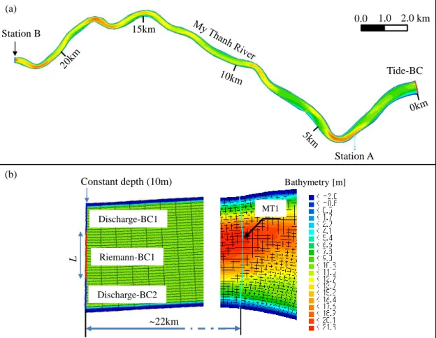
This study was conducted in My Thanh River, the main tidal river of Soc Trang province that lies off the East coast of Southern Vietnam (Figure 1-1 and Figure 1-2). This river drains directly to the East Sea (South China Sea), and the upstream bifurcates into two main channels and a complex canal network toward the in-land area. Its upstream also connects to the Hau River (Bassac River), so its flow regime is under the multi-influence of the semidiurnal tidal regime of the East Sea, Hau River, and upstream channels. Many people are living near the riverbank by doing agriculture and aquaculture. This river was selected because it can represent other small tidal rivers in VMD.

Only tidal data at My Thanh station are available but only from 1985 to 2007. After this period, this station was already stopped but tidal data at Tran De station at Bassac estuary, about 10 km from the old station (Figure 1-1) can be used. However, in this study, the tidal data at Tran De station could be found only from 2008 to 2014.

(15)

5

Figure 1-2. My Thanh River with field observation overall planning (a), and equipment setup (b).

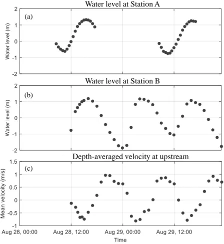
Besides, two same field measurement campaigns were conducted in My Thanh River on 16th_{, 17}th_{June, and 28}th_{, 29}th_{August 2018 to collect necessary field data. The}

measurement length is approximately 22km from the estuary. Figure 1-2 (a) depicts the layout of these measurements to collect hydraulic data of My Thanh River such as discrete depth samples, discharge and velocity, and water level. In each campaign, two teams were needed to run these measurements. The first team operated the Boat 1 across the river at the upstream location every hour to get water velocity and discharge by using an ADCP device installed on the boat as in Figure 1-2 (b). Simultaneously, the other team operated the Boat 2 along the river to collect the discrete depth samples also by an ADCP. Boat 2 followed a zigzag trajectory as shown by the red line in Figure 1-2 (a). Additionally, half-hourly water level data were also recorded manually at two observation locations Station A and Station B by using rulers. The measured data in June and August 2018 were used for validation and calibration of the 2-D flow model of My Thanh River, respectively.

1.4 Thesis outline

This thesis is comprised of six chapters that include the introduction (Chapter 1) and conclusions (Chapter 6). The body chapters (Chapters 2 to 5) follow the research objectives indicated above.

Chapter 2 shows the overall review of the related studies, including hydrodynamic

models and its applications, modeling the flow of small tidal rivers using Riemann Boundary, and river topography interpolations.

Boat 1 Boat 2 Upstream Station B Station A My Thanh Station 2km Computer with Winriver II software ADCP (a) (b)

(16)

6

Chapter 3 presents a new searching method for finding samples to estimate the

bathymetry of rivers which can be combined with common interpolators to estimating three-dimensional (3-D) river shape from sparse zigzag depth data. It has been shown to be excellent in shape estimation near the riverbank, especially in curved areas.

Chapter 4 describes a 2-D flow model of the study river which is applied the Riemann

boundary condition proposed by Takagi et al. (2019) is improved by considering the flow velocity loss near the riverbank, and the boundary condition at the upstream end is given.

Chapter 5 concentrates on improving the 2-D flow model in Chapter 4 by reviewing the

tidal level measured at the river mouth and nearby station, and the model was calibrated and optimized using the spatio-temporal velocity records measured by ADCP device to significantly improve the reproducibility of the flow field.

(17)

7

Chapter 2 Literature review

2.1 Hydrodynamic model

Hydrodynamic models are applied to illustrate the flow field as direction and magnitude, and depths of the river for various conditions of flow. Hydrodynamic modeling can be classified into three main groups based on the used equations and the computational domain, including: one-dimensional (1-D), two-dimensional (2-D), and three-dimensional (2-D).

2.1.1 1-D Hydrodynamic model

1-D model is the simplest option that describes the flow conditions within a river by a set of cross-sections. The simplest form of the 1-D model solves one-dimensional energy equations to compute water-surface elevations at each cross-section for steady gradually varied flow conditions. A slightly more sophisticated 1-D model simulates unsteady-state flow conditions in river channels and solves cross-sectional averaged Saint-Venant equations to route the flow hydrograph and compute water surface elevation at each cross-section. There are some common 1-D models, such as HEC-RAS (USACE, 2016b) from U. S. Army Corps of Engineers, MIKE 11 (DHI, 2017a) from the Danish Hydraulic Institute.

1-D models are suitable for modeling hydraulic structures such as bridges, culverts, gated spillways, weirs, drop structures, as well as lateral structures (USACE, 2016b). However, they are not specialized for modeling 2-D features such as the spatial distribution of flows, meander, flooding in the catchment area.

The 2-D hydrodynamic model solves depth-averaged mass and momentum equations to compute water-surface elevations and velocities at any point of used finite element grid. At each point, three values are computed including water depth, and velocities in two directions (i.e. x and y directions). The vertical accelerations of 2-D models are negligible. The velocity vectors are assumed to point in the same direction over the entire depth of the water column. There are some commonly used 2-D hydrodynamic models, such as

(18)

8

MIKE 21 (DHI, 2017b) from the Danish Hydraulic Institute, Delft3D (Deltares, 2017) from WL|Delft Hydraulics and Delft University of Technology, HEC-RAS 2D Modeling (USACE, 2016a) from U. S. Army Corps of Engineers. To implement a 2-D model, some typical data are required, such as bathymetric data, boundary conditions, and calibration data.

The most common boundary condition types of the 2-D model are water level at downstream and water discharge at upstream. Calibration data mainly based on point measurements of water level, velocity, and discharge. Various combinations were used, for example using only water level (Pham Van et al., 2016; Ijaz et al. 2019), water level and discharge (Islam et al., 2018; Xie et al., 2019), water level and velocity (Zarzuelo et

al., 2019). These measurements are compared with model computations, and the

parameters of the model are adjusted to improve the match of its results and measured values. Spatial calibration was also considered due to the complexity of river flow; however, recently spatial calibration was restricted in using velocity data along only one cross-section besides other data (Elias et al., 2012).

The accurate description of river bathymetry is an important factor in the accuracy of the 2-D model. The river bathymetry represents the spatial variations in the riverbed by specifying the bed elevation at every node of the finite element grid of the computational domain. 2-D models were also found to be very sensitive to river bathymetry (Bovee, 1996). Therefore, the accuracy of the 2-D model is highly dependent on the accuracy of river bathymetry and the characteristics of the used finite element grid.

3-D model is similar to the 2-D model, except that the governing equations are not depth-averaged. The number of layers in the water column is defined as the third dimension or vertical dimension (z) of the model besides the two horizontal dimensions (x and y). Hence, the 3-D model is suitable to describe the vertical profiles of flow and velocity as stratification, diffusion, and dispersion processes throughout the modeled area. The 3-D model thus consumes more computational time and requires more storage volume than the 2-D model. However, with the development of computer technology today,

(19)

9

computational time and storage volume may not be a big concerning issue with the 3-D model.

The 3-D model requires similar input data to the 2-D model. However, the measurements of velocity fields in the vertical direction are necessary for open boundary conditions and calibration of models (Fissel et al., 2002). The accuracy of the river bathymetry is also an issue of the 3-D model.

2.1.4 The applications of hydrodynamic models

Hydrodynamic models hold a crucial role in investigating fluvial processes such as sediment transport, morphological changes, bank erosion, salinity intrusion, or flooding and risk. The followings are some selected studies related to these applications.

Coupling with sediment transport and morphological model, the hydrodynamic model is a very convenient process-based method to study sediment transport and morphological changes. The 2-D model is commonly coupled with sediment transport and morphological model to simulate the transport of cohesive/non-cohesive suspended sediment and/or morphological changes in river channels or coastal regions (van der Wegen et al., 2011; Bi and Toorman, 2015; Xie et al., 2018), the morphodynamic response of a tidal estuary inlet to sea-level rise (Yin et al., 2019). The 3-D model is also coupled with sediment transport and morphological model to investigate sediment dynamics and morphodynamic changes in the estuaries and coastal zone (Thanh et al., 2017; Tu et al., 2019). Key factors that strongly influence the distribution and transport of suspended sediment, erosion/deposition patterns were investigated.

Hydrodynamic models are also useful for simulating riverbank erosion. The 1-D model and sediment transport model was coupled with a 2-D model of groundwater flow and a riverbank erosion model for investigating the mechanism of the cantilever failure of a composite riverbank (Deng et al., 2019). The 2-D model and sediment transport model was coupled with groundwater flow and bank stability analyses to access the influence of hydraulic erosion on mass failure processes (Rinaldi et al., 2008), with a process-based bank stability model to predict bank retreat (Lai et al., 2015), or with geotechnical and vegetation module to simulate the riverbank erosion (Rousseau et al., 2017).

(20)

10

Both 2-D and 3-D hydrodynamic models are applied to study salinity intrusion, but 3-D models are more common because of the capacity of describing detailed flow information. Thanh et al. (2017) and Tran Anh et al. (2018) successfully simulated salinity concentration in the Hau River (Vietnam), focusing on the salinization-prone section between Can Tho, Dinh An, and Tran De estuaries by coupling the 2-D model with salinity transport model. Besides, the 3-D model was also successfully combined with the salinity transport model to analyze the characteristics of salinity intrusion (Jeong et al., 2010) or to quantify the influences of sea-level rise on saline water intrusion (Hong and Shen, 2012; Chen et al., 2016).

A 2-D hydrodynamic model is also a good tool for investigating storm surge or flooding and risk. The 2-D model could be regularly incorporated with a wave model to simulate cyclones and analyze the attenuation role of mangroves within coastal environments (Rahdarian and Niksokhan, 2017), estimate hydrodynamic and morphological responses of the long-narrow estuary to a major storm (Kuang et al., 2020). The 2-D model is also applied to assess the flood regulation function of paddy fields (Hai et al., 2006), or investigate the local amplification of flow velocity in narrow river channel which is helpful information in evaluating flood/inundation risks in urban areas in the VMD (Takagi et al., 2016b). The 1-D model is also used to analyze the characterization of the historical flood hazard, vulnerability, and risk and forecast the future hazard due to the projected sea-level rise in the VMD (Van et al., 2012; Tri et al., 2013).

2.2 Hydrodynamic models of tidal rivers using Riemann Boundary

As mentioned above, the upstream open boundaries of 2-D/3-D hydrodynamic models of rivers are commonly configured using measured river discharge. However, modeling works are often experienced with insufficient historical discharge data problems, so it is hard to describe an upstream open boundary of the flow model. Takagi et al. (2019) introduced a simplified methodology for modeling the flow of a large tidal river without discharge at the upstream boundary; the driving force is mainly produced by the variation of ocean elevation at the downstream open boundary. In this simplified model, the upstream boundary was applied to a Riemann Boundary, which enables progressive waves to pass through the boundary without reflection. The Riemann Boundary was also

(21)

11

demonstrated that it is convenient for setting up the upstream boundaries of not only river channels but also small tributaries (Takagi et al., 2016b).

2.3 River topography interpolation

2.3.1 Bathymetric survey

Sciortino (2010) referred to a bathymetric survey as a hydrographic survey that measures the water depth of the river or ocean to produce the bathymetric map. In this activity, two measurement works are implemented simultaneously, including vertical depth and horizontal position measurements. These measurements can be supported by either manually (low tech, low cost) or sophisticated depth and position equipment (high tech, high cost), depending on the purpose of the survey. The vertical depth can be measured by a simple engineering echosounder or an advanced echosounder which can communicate with computer software to record the water depth data as ADCP, single or multibeam Sound Navigation And Ranging (SONAR) devices. The horizontal positions can be collected by various methods such as a floating line, theodolite, a Global positioning system (GPS), or a differential GPS (DGPS). ADCP devices are suitable for surveying the river cross-sections. SONAR devices are very convenient for the bathymetric survey, very high-resolution output data can be exported directly into the bathymetric map of the river or ocean. However, SONAR devices are suitable for large and relatively deep rivers.

Nowadays, many remote sensing techniques have been preferred for bathymetric mapping as Airborne bathymetric LiDAR (Hilldale and Raff, 2008), spatial depth, and through-water photogrammetry (Shintani and Fonstad, 2017). These methods allow a rapid survey of large areas and can be operated over a wide range of water depths in clear water, but their operations are strongly affected by various environmental factors such as water clarity, surface waves; the surveying cost is also very high because these devices must be mounted on planes or helicopters (Kasvi et al., 2019).

Hydrographic data was measured and stored in different ways such as cross-sectional, random, zigzag, or very high-resolution distribution depending on the purposes or applying methods of the measurement works. Cross-sectional distribution is the most

(22)

12

common distribution of hydrographic data because it can describe effectively the anisotropy of riverbed. However, the distance between adjacent measured cross-sections should be close together to provide adequate information about the bottom features of the interested rivers, the recommended distance is 0.5 or 1 times the average river channel width to ensure that the interpolated bathymetry can capture sufficient major topographic features (Conner and Tonina, 2013).

2.3.2 Bathymetric interpolation

Bathymetric data play an important role in the 2-D/3-D flow model which shows detailed information of riverbed. Estimating river channel topography has been concerned by researchers in recent years. More than 40 different spatial interpolation methods were investigated and classified into two main groups including deterministic and geostatistical methods (Li and Heap, 2008). The deterministic interpolators estimate the value of unmeasured location by mathematical functions on the surrounding measured values. The interpolators, such as Triangular Irregular Networks (TIN), Inverse Distance Weighting (IDW), Radial Basis Function (RBF), and Local Polynomial Interpolation (LPI) are classified as deterministic methods. Conversely, the geostatistical methods apply both mathematical and statistical models that describe autocorrelation or statistical relationships between different measured points. Kriging interpolators were known as geostatistical methods.

The anisotropy of riverbed is very important information in interpolating the river bathymetry (Burroughes et al., 2001; Goff and Nordfjord, 2004). This is a crucial viewpoint of customized or modified interpolation methods. Modified interpolation methods are commonly applied to IDW than other methods because it is simpler to implement. Burroughes et al. (2001) developed a zonal inverse distance weighting (Z-IDW) which recognizes and separates the estuary into some different zones based on the depth range to specify inverse distance weighting for each area separately. Modifying the searching method to consider the anisotropy of river channels is another approach to customize the IDW method. Merwade et al. (2006) introduced an elliptical inverse distance weighting (E-IDW) which involved measurement samples by an elliptical box followed the flow direction in a flow-oriented (s, n) coordinate system instead of a circular box to include the anisotropic nature of the channel while interpolating the river channel

(23)

13

bathymetry. Similarly, Andes and Cox (2017) applied a rectangular box followed the flow direction to define the rectilinear IDW (R-IDW) method. These modified interpolators indicated the ability to improve the estimated bathymetry of rivers.

Ordinary Kriging (OK) method is also applied to interpolate the river channel bathymetry. Carter and Shankar (1997) found that the OK method is unable to handle a trend in the data and suggested that the dominant trend should be removed from measured data before applying OK interpolator. Merwade et al. (2009) suggested a method to estimate the surface trend of the river bottom and remove it before making interpolation; this trend, finally, was added back to the estimated result to obtain the final bathymetry. This method improved significantly the estimated river topography.

2.4 Demand for deploying a 2-D flow model and estimating river bathymetry from sparse depth data for small tidal rivers in the VMD

Although the 2-D hydrodynamic model only estimates the depth-averaged velocity of a river, it is very effective to investigate the mechanism of most of the fluvial processes as sediment transport, riverbank erosion, riverbank retreat, salinity transport, storm surge, or flooding and risk. A 2-D model is also easy to upgrade to a 3-D model by adding vertical layers and collecting water velocity over the water column. Hence, modeling the 2-D model of a small tidal river is the first crucial step before investigating the mechanism of other fluvial processes to deal with related problems.

In the VMD, besides the large river system, most of the small tidal rivers are almost lack of hydrodynamic data so the simplified methodology of Takagi et al. (2019) is very helpful to conduct their 2-D flow models. However, this method is still in its infancy because it neglects some important characteristics affecting hydraulics in the estuarine environment. Further improvements should be considered to make this method more reliable and applicable to the small tidal rivers in the VMD.

The modern techniques are difficult to apply for surveying the topographic data of small tidal rivers in the VMD because they are generally deep and have very high turbidity. Although the ADCP-based method is also facing many dangers as the high speed of water flow, obstacles from fishing activities, or heavy traffic conditions in some rivers; it is the

(24)

14

most suitable method to apply in the VMD. However, the surveying boat should be tried to follow other strategies that are more flexible and faster than the cross-section strategy to be suitable for the local conditions in the VMD.

Many interpolation methods have been concentrated on improving the quality of river topography by involving the anisotropy of the riverbed. Most studies mainly deal with meandering and applied on cross-sectional data; lack of studies concentrated on other kinds of topographic data such as zigzag distribution data or improving the estimated depth at near riverbank areas which are important for studies as riverbank erosions or riverbank failures. Therefore, new interpolation methods that can be applied to zigzag data and improved the estimated depth near riverbank areas are really helpful for studying the small tidal rivers in the VMD.

(25)

15

Chapter 3 Interpolation of the river bathymetry based on sparse depth

data

A Curvilinear search method is proposed as an interpolation search method for reproducing a three-dimensional river shape with sparse zigzag depth data. This method, combined with IDW, OK, and RBF interpolation, is optimal for estimating 3-D river shape from sparse zigzag depth data. It is excellent in shape estimation near the riverbank, especially in curved areas.

3.1 Introduction

Bathymetric data play an important role in river numerical modeling works. Most of the small tidal rivers in the VMD are lack of bathymetric data. Deploying modern equipment as LiDAR or remote sensing technology to measure high-resolution depth data to export directly the bathymetry might be difficult because rivers in this region are generally deep and have very high turbidity. The literature review in the previous chapter indicated that many studies have focussed on improving the quality of interpolated bathymetry by taking the anisotropy of riverbed into account. However, these studies mainly applied to cross-sectional or random distribution data which are difficult to measure in the VMD because of high water speed, heavy traffic load, and many obstacles from the fishing systems of local people. Hence, other kinds of depth data as zigzag data should be considered to make the field works easier in the VMD.

Estimating unmeasured depth locations by involving samples along the flow direction is the common solution to consider the anisotropy of the riverbed (Merwade et al., 2006; Andes and Cox, 2017). As stated in the literature, E-IDW and R-IDW are operated in (s, n) coordinate system to deal with meandering rivers and data-point anisotropy. These methods worked effectively with rivers whose widths are not complex and distances between adjacent cross-sections are short (i.e. 0.5 or 1 times the average river channel width as mentioned by Conner and Tonina (2013)). If the distances between two adjacent become larger or rivers are not straight (i.e. in flow-oriented (s, n) coordinate system), the searching boxes (ecliptical or rectilinear box) of these methods unfollow the flow direction when finding the samples near the riverbank areas. Therefore, the estimated

(26)

16

depth near the riverbank, in this case, will be under-estimated. Hence, a new searching method should be proposed to account for this problem and optimize the near riverbank estimated topography.

Thalweg-line-based interpolations are other methods that effectively coped with riverbed anisotropy. Caviedes-Voullième et al. (2014) used the thalweg and two bank lines as break-lines to generate the interior splines parallel to the main flow direction and the depths along them are estimated by the linear method. Chen and Liu (2017) also manipulated three break-lines to distinguish the river channel but into four separated regions before resampling existed cross-sections and estimating extra cross-sections by various interpolators. Similarly, Lin et al. (2018) also divided the river into two regions by the thalweg and applied linear methods to estimate extra points for measured cross-sections and un-measured depths in the longitudinal direction. These interpolation methods obtain good estimation; however, the thalweg line is only specified effectively by cross-sectional data with short adjacent distances. Consequently, these methods are difficult to apply with sparse cross-sections or zigzag distribution data because it is difficult to estimate the thalweg line from them.

Zigzag distribution data are uncommon in river topography investigation because they are unable to describe well the transverse profiles of rivers and has many large areas lack of depth information. Krüger et al. (2018) proved that surveying strategies or sampling methods have a great influence on the quality of the interpolation results, and zigzag distribution data are also suitable for estimating the river topography. However, in this work, the zigzag data in double and ideal distribution were exported from very high-resolution data. In the VMD, most rivers are very deep, high flow speed, high traffic load, having many obstacles from fishing activities of local peoples so the zigzag strategy should be applied to measure the topographic data because it is very flexible and easy to operate in comparing with cross-sectional strategy.

In this study, the zigzag strategy was applied to acquire the hydrographic data of the study river and a new searching method was proposed to estimate the bathymetry from these measured depth data. The proposed searching method was guaranteed that involved samples follow the longitudinal direction regardless of the distance from the interpolation

(27)

17

location to them, estimating depth in the middle of the river or near the riverbanks. The proposed method was also compared with other searching methods by applying them with three common interpolators, including IDW, OK, and RBF method. Estimated bathymetries were also carefully compared to figure out which methods are suitable for similar studies in the future. All tasks in this study have been implemented on the Matlab environment instead of a geographic information system (GIS) software and output bathymetries could be directly applied for modeling the 2-D/3-D flow model of rivers by using Delft 3D software.

3.2 Methodology and data

3.2.1 Depth samples data

Exported depth samples from ADCP data by using WINRIVER II software are referred on the water-surface elevation. The water-surface elevation must be converted to the Vietnam National Datum (VN-2000) by using the nearest data contributed by the local government. Figure 3-1 shows the procedure jointing the VN-2000 water level at Station A with ADCP depth data to produce the VN-2000 discrete depth samples. In the procedure, the spatial distribution of water level across My Thanh River is assumed to be constant and equals with the water level at this station.

Figure 3-1. Convert ADCP data to depth samples. Water level data

at Station A (VN2000 Datum) River depths

(referenced to water surface)

Depth data points (VN2000 Datum) Measured time (hh:mm) Water level (at measured time) ADCP Data

(28)

18

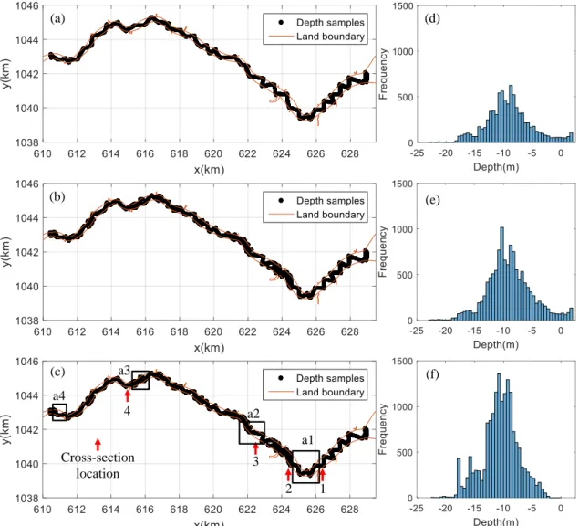
Figure 3-2. Distribution of classified depth sample data: calculating data (a, b) and calibrating data (c, d); and histogram graphs of their depth (c, d, f).

The depth samples in June with some selected samples in August were applied for interpolation study. The combination data were split into two groups, including calculating data for estimating the river bathymetry and testing data for validating applied interpolators. The calculating data are divided into two sub-groups, including (1) only zigzag samples (Figure 3-2 (a)), and (2) zigzag samples with some additional samples (Figure 3-2 (b)); the testing data include spatially distributed and four cross-sectional samples as shown in Figure 3-2 (c). The histograms of these groups show that the common depth of My Thanh River is about 11 m, with the deepest location is about 23 m (Figure 3-2 (d), (e), (f)). (a) (c) (e) (b) (d) (f) 4 3 2 1 Cross-section location a1 a2 a3 a4

(29)

19 3.2.2 Searching methods

The elliptical search (Merwade et al., 2006) and rectilinear search (Andes and Cox, 2017) were improved the estimated river bathymetry significantly. However, these methods only work effectively with rivers which are nearly constant in width. In the case of river width highly changes, both elliptical and rectilinear search will have a common problem as shown in Figure 3-3. Obviously, in-stream samples at A in Figure 3-3 and near riverbank samples B will be included for interpolating at an in-stream unknown depth location C. This will generate more errors due to the certain change of the depth along the river cross-section. The searching box in this case has also not followed the river flow. To account for this problem, a new searching strategy was implemented as illustrated in Figure 3-3. This method works directly with the curvilinear grid of the study area in (x, y) Cartesian coordinate system. Figure 3-3 shows that the depth at the current grid node (ith, jth) is calculated by using depth samples on the left and the right of this node. These samples were found by sliding a searching box to both sides of the current node. The size of the box can be defined by users. The red curvilinear box in Figure 3-3 represents the trajectory of curvilinear search near the riverbank and in the area where river channel width changes significantly. Curvilinear search can be applied to derive new modified versions of common interpolation methods as IDW, OK, and RBF, so-called IDW, C-OK, and C-RBF (i.e. C stands for the Curvilinear search), respectively, for estimating riverbed topography using a sparse zigzag or cross-sectional dataset. Besides, the rectilinear search and the nearest neighbor search were also applied with these methods to derive six other methods including R-IDW, R-OK, R-RBF, NN-IDW, NN-OK, and NN-RBF with R and NN are represent for rectilinear and the nearest neighbor searches, respectively. All interpolators were applied to estimate the bathymetries of My Thanh River using the zigzag dataset to find out the suitable methods.

(30)

20

Figure 3-3. Previous and proposed searching methods.

3.2.3 Interpolation methods

IDW is a well-known deterministic interpolation method that can estimate the value of an unsampled location by a linear combination of involved samples (Li and Heap, 2008). The distances from involved samples to the unknown location are put in evaluating the impact of their values to the interpolated result by the following equation:

𝑧̂(𝑥₀) =∑ (𝑑𝑖 −𝑝 𝑧(𝑥𝑖)) 𝑁 𝑖=1 ∑𝑁_𝑖=1𝑑_𝑖−𝑝 (1)

where 𝑧̂(𝑥₀) denotes the estimated value at an unknown location 𝑥₀, 𝑧(𝑥_𝑖) is the value at the ith location, N is the number of included samples, di is the distance between x0 and xi,

and p is the weighting power.

Similar to IDW, the RBF method also use the distances from included samples to interpolated location. However, RBF is a radial basis function network (RBFN) using these distances as inputs of its activation function to estimate the value of an unsampled location (Lin and Chen, 2004). The activation function is a nonlinear function that is radially symmetric in the input space. The RBF estimator equation as following:

Depth samples Centre line Riverbank Rectilinear search Proposed search -250 -200 -150 -100 -50 0 50 100 150 200 250 17.8 ₁₈ _18.2 _18.4 _18.6 _18.8 n co o rd in ate (m ) s coordinate (km) A C B

(31)

21

𝑧̂(𝑥0) = ∑𝑁𝑖=1𝑤𝑖𝜑(‖𝑥0− 𝑥𝑖‖) (2)

with wi is the weight coefficients computed by solving the following linear system:

[ 𝜑(‖𝑥₁− 𝑥₁‖) 𝜑(‖𝑥2− 𝑥1‖) 𝜑(‖𝑥₁− 𝑥₂‖) 𝜑(‖𝑥2− 𝑥2‖) ⋯ 𝜑(‖𝑥_𝑁− 𝑥₁‖) … 𝜑(‖𝑥_𝑁− 𝑥₂‖) ⋮ ⋮ 𝜑(‖𝑥1− 𝑥𝑁‖) 𝜑(‖𝑥2− 𝑥𝑁‖) ⋱ ⋮ … 𝜑(‖𝑥𝑁− 𝑥𝑛‖) ] [ 𝑤₁ 𝑤₂ ⋮ 𝑤_𝑁 ] = [ 𝑧(𝑥₁) 𝑧(𝑥₂) ⋮ 𝑧(𝑥_𝑁) ] (3)

where 𝜑(𝑟) = 𝜑(‖𝑥𝑖 − 𝑥𝑗‖) is the activation function. There are many kinds of

activation functions such as the thin-plate-spline function, the Gaussian function, the multiquadric function, and the inverse multiquadric function (Chen et al., 1991). In this study, however, only the multiquadric function was applied, its formulation as following (𝜎 is a constant):

𝜑(𝑥_𝑖− 𝑥_𝑗) = √1 +(𝑥𝑖−𝑥𝑗)2

𝜎2 (4)

The OK method is a kind of geostatistics interpolator estimated the unknown value by using the spatial correlation between collected samples (Li and Heap, 2008), the OK estimator equation as following:

𝑧̂(𝑥₀) = ∑𝑁 𝜆_𝑖

𝑖=1 𝑧(𝑥𝑖) + [1 − ∑𝑁𝑖=1𝜆𝑖]𝜇(𝑥0) (5)

where 𝜆𝑖 is Kriging weights and ∑𝑁𝑖=1𝜆𝑖 = 1, and 𝜇(𝑥0) is the local mean of samples

within the search box. The Kriging weights are computed by the following linear system:

[ 𝐶(𝑥₁, 𝑥₁) 𝐶(𝑥₁, 𝑥₂) 𝐶(𝑥₂, 𝑥₁) 𝐶(𝑥₂, 𝑥₂) ⋯ 𝐶(𝑥₁, 𝑥_𝑁) 1 … 𝐶(𝑥₂, 𝑥_𝑁) 1 ⋮ ⋮ 𝐶(𝑥𝑁, 𝑥1) 𝐶(𝑥𝑁, 𝑥2) 1 1 ⋱ ⋮ ⋮ … … 𝐶(𝑥₁𝑁, 𝑥𝑁_{0 ]}) 1 _[ 𝜆1 𝜆2 ⋮ 𝜆_𝑁 𝜇(𝑥₀)] = [ 𝐶(𝑥₀, 𝑥₁) 𝐶(𝑥₀, 𝑥₂) ⋮ 𝐶(𝑥₀, 𝑥_𝑁) 1 ] (6)

where C is a covariance function describing the spatial correlation between referenced samples, and C is calculated from the semivariogram model of samples.

(32)

22 3.2.4 Implementation of interpolation methods

Most procedures in this study were developed in a Matlab environment. Figure 3-4 describes the algorithm of the MATLAB program which follows several steps. At first, the curvilinear grid of My Thanh River was created separately by using the RGFGRID tool (Deltares, 2020b) and converted to Matlab structure data by using the QuickPLOT tool (Deltares, 2014b). This structure data contains the (x, y) Cartesian coordinates of the computational grid where the depths will be estimated. Next, the structure data and all kinds of depth samples were imported to Matlab as input data. After that, all searching methods were used to find samples for interpolating the depth at the current grid node (ith, jth). The IDW, RBF, and OK methods were implemented based on the equation (1), (2), and (3), respectively. The RBF and OK method applied exist MATLAB libraries which were developed by Chirokov (2006) and Ramm (2011), respectively. Ramm (2011) developed this library mainly based on the Gstat package (Pebesma and Wesseling, 1998). However, IDW was written by the author it is easy to implement. The mean absolute errors (MAEs) of predicted bathymetries were calculated to access the quality of output bathymetries. If MAEs of any methods are large, the parameters will be modified and run the program again. No specific criteria for MAEs, the try-and-error method was applied to reduce the errors as much as possible. Finally, the final bathymetries will be exported into the DEP-extension file (Deltares, 2014a), which are ready for 2-D/3-D flow modeling.

(33)

23

Figure 3-4. Flowchart of interpolation Matlab program.

3.3 Results and discussions

3.3.1 Comparing surfaces

To assess the influence of samples density and determine which interpolation methods are suitable with the zigzag dataset, the MAE between estimated bathymetries and testing dataset (Figure 3-2 (e)) were calculated by the following equation:

MAE = 1

N∑ (𝑧̂𝑖 − 𝑧𝑖) 𝑁

𝑖=1 (7)

where N is the number of testing depth samples, 𝑧̂_𝑖 and 𝑧_𝑖 are the estimated and measured depth at the ith location, respectively.

The MAE values of estimated bathymetries shown in Table 3-1 indicate that NN-IDW, NN-OK, and NN-RBF method resulted in a large discrepancy from the testing data (greater than 1 m), while C-IDW is the best suitable method with the lowest MAE values in both cases of testing data. Additionally, with the same interpolators, curvilinear search

(ith, jth) grid node

Curvilinear search

Depth samples

Curvilinear grid

Raw depth exported from ADCP data

Searching samples (Rectilinear, curvilinear, nearest neighbor search)

Estimate the depth at (ith,

jth) grid node

Estimated all nodes?

Switch to the next node RGFGRID Tool QUICKPLOT Tool Curvilinear grid Matlab Environment No Yes Save the bathymetry

Included samples

Matlab structure of grid Calculating samples

(34)

24

always generated better bathymetry than others. It means that curvilinear search is the most suitable searching method working with the zigzag distribution samples. Moreover, increasing the density of samples the predicted bedforms were improved, and it is an unsurprising result because more samples caught more bottom features; this is consistent with the study of Diaconu et al. (2019) instead of differences in the spatial distribution of samples.

Table 3-1. Calculated MAE of estimated bathymetries.

MAE (m) Calculation cases

Interpolation methods Case 1 Case 2

C-IDW 0.60 0.55 C-OK 0.70 0.65 C-RBF 0.61 0.56 R-IDW 0.63 0.59 R-OK 0.81 0.73 R-RBF 0.77 0.68 NN-IDW 1.58 1.46 NN-OK 1.19 1.17 NN-RBF 1.21 1.11

(35)

25

Figure 3-5. The estimated depth of C-IDW and R-IDW interpolator at four areas marked from a1 to a4 in Figure 3.2, and extracted depth profiles of four selected cross-sections

from CS-a1 to CS-a4 in these areas. In the case of CS-a2, its location is near Cross-section 3, so the estimated depths were extracted at the measured locations.

To present the problem of rectilinear search at the near riverbank, four potential areas in the My Thanh River were selected and marked from a1 to a4 as shown in Figure 3-2(c). The estimated bedforms of these areas are displayed in Figure 3-5, the first row and second row were estimated by R-IDW and C-IDW, respectively. The bedforms in the first row look abnormal and unnatural; the shallow bars and deep areas near riverbanks are the results of involving unsuitable depth samples for interpolating. Similarly, the R-OK

R-IDW C-IDW a1 a2 a3 a4 Shallow bar Deep area near riverbank

(36)

26

method also has the same problem with R-IDW because the OK method also manipulated directly the depth values, while the RBF method used the distances. Nevertheless, the bedforms estimated by C-IDW are very smooth and natural. Hence, the curvilinear search has already improved the estimated bathymetry but mainly in near-bank regions, while the middle area is very consistent with R-IDW. Exported cross-sectional profiles of CS-a1 to CS-a4 are clearly to show that C-IDW cross-sections are very smooth in comparison with R-IDW cross-sections.

Figure 3-6. The regional MAEs of using interpolators calculated at near riverbank areas (a) and the middle area of the river (b), the red-dash boxes show the suitable

interpolators in this region.

However, the regional MAEs calculated by estimated bedforms and testing data reveals other interesting results. Adding more samples has only refined the estimated depth at the near riverbank areas, the MAEs notably decreased in all cases (Figure 3-6 (a)), while slightly changed in the middle of the river (Figure 3-6 (b)). Figure 3-6 indicates that C-IDW, C-OK, R-C-IDW, and R-OK methods are suitable to reproduce the depth of the middle river, while only C-IDW and C-OK are suitable for the near riverbank areas.

0 0.5 1 1.5 2 2.5

IDW OK RBF IDW OK RBF IDW OK RBF Curvilinear Rectilinear Nearest neighbor

E rr o r (m )

MAE of the near banks area

Case 1 Case 2 0 0.5 1 1.5 2 2.5

IDW OK RBF IDW OK RBF IDW OK RBF Curvilinear Rectilinear Nearest neighbor

E rr o r (m )

MAE of the middle area

Case 1 Case 2

(a)

(37)

27

Consequently, two groups of interpolation methods can be applied to predict the river bedform based on zigzag depth samples. The first group is the interpolators working with curvilinear search (C-IDW, C-OK, C-RBF) and R-RBF method. C-IDW is the best method. The second group is regional interpolators which are the C-IDW method for estimating the near riverbank areas combining with C-RBF or R-RBF method for estimating the middle river area, respectively.

3.3.2 Comparing cross-sections

The error of estimated depth was calculated by the following equation

e_i = 𝑧̂_𝑖 − 𝑧_𝑖 (8)

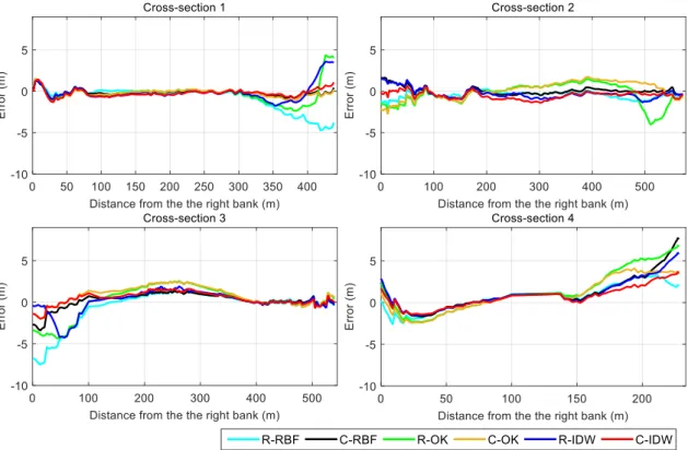
where, 𝑧̂𝑖 and 𝑧𝑖 are the estimated and measured depth of the ith sample. Figure 3-7

illustrates the error profile of four selected cross-sections named from 1 to 4 as shown in Figure 3-2 (c). Especially, Cross-sections 1 and 3 are situated in areas a1 and a2 where the estimated bathymetries generated R-IDW method has a problem, therefore they are effective to compare the performance of interpolation methods. Generally, the primary differences occur at near riverbank areas except Cross-sections 2 and 3 where the OK method has larger errors in the middle. The interpolation methods working with curvilinear search could generate a better cross-sections profile than them working with rectilinear search except for the IDW and RBF method at section 2 and Cross-section 4, respectively (Table 3-2). The mean MAEs show that C-IDW is the best method. Particularly, interpolation methods worked with rectilinear search reconstructed worse depths at the left bank and the right bank of Cross-sections 1 and 3, respectively, than with curvilinear search; it reconfirmed the drawback of the rectilinear search. Located in the straight river where the topography is not significantly changed, the depth profile of Cross-section 2 was estimated well, but the R-OK method underestimated the depth near the left bank. It may be occurred by the semivariogram model was not described well the spatial correlation in this area. The depth profile of Cross-section 4 is the most difficult to predict, especially at the left bank, because it is located at a complex meandering where the topography is rapidly changed. No methods operated well at this bank except the C-IDW.

(38)

28

Figure 3-7. Error profiles of estimated depths by applied interpolators at four cross-sections, their locations are marked in Figure 3-2.

Table 3-2. Calculated MAE of four reproduced cross-sections.

MAE (m) Cross-section 1 Cross-section 2 Cross-section 3 Cross-section 4 Mean MAE C-IDW 0.28 0.54 0.88 2.77 1.12 R-IDW 1.12 0.53 1.78 5.84 2.32 C-OK 0.28 1.04 1.95 6.65 2.48 R-OK 1.29 2.05 3.75 11.40 4.62 C-RBF 0.17 0.75 1.00 8.19 2.53 R-RBF 2.76 4.97 5.28 3.19 4.05

(39)

29 3.3.3 Discussions and future works

The demand for estimating an accurate bathymetry has been remained because of the crucial role of bathymetric data in the numerical model. This study not only indicated the effectiveness of curvilinear search but also figured out the suitable methods which can work well with the sparse depth dataset collected by zigzag strategy. This is a fast, flexible, easy-to-setup strategy, and very convenient to apply for rivers in the VMD.

Difficulties of estimating depth for the near-bank regions are mainly caused by insufficient depth data (Andes and Cox, 2017; Hilton et al., 2019). Hilton et al. (2019) suggested using modern equipment (i.e. ATLAS, LiDAR, ICESat-2) to collect more data. However, these systems might be not operated well with rivers in the VMD because of the deep and high-turbidity water. So, the proposal of the curvilinear search is the first step to improve the estimated depth of these areas. Besides, our study also ensures that the predicted bathymetry is ready for flow modeling. The main factor to have this ability is that our algorithm used directly the computational grid of the numerical model. Andes and Cox (2017) and Hilton et al. (2019) concluded that their output bathymetries were also ready for flow modeling, but they did not clearly show how to archive this. However, our method has only validated with the curvilinear grid, other types of the grid such as unstructured grid or grid from other numerical tools should be supported in the future. Similar to the cross-section strategy, the zigzag strategy also can not measure the depth of the near riverbank areas because of the limitation of the navigation. To deal with this handicap, the riverbank elevations at the land boundary were assumed 2 m (VN-2000 datum). After that, additional samples were generated at some locations where have the shortest distance to the riverbank by using the linear method. This method was already applied by Falcão et al. (2016) to combine the estimated river bathymetry and floodplain area. However, it is better to find a new way to estimate the bathymetry for these areas in the future, such as analyzing the satellite images, drone-based remote imaging at the lower-low-water (LLW) period of the tide, scanning depth by a sonar sensor, or generating depth by combining the cross-section tendency and small random-depths represented for the roughness of the riverbank.

(40)

30

Our interpolation results revealed that the depth of the middle river is estimated easier than that of near-bank areas, it is consistent with the results of Andes and Cox (2017) and Hilton et al. (2019). It implies that a mixed-method joining between methods operated well in the near-bank and methods worked well in the middle river areas should be applied to have the best bathymetry. This study already proposed such kind of methods. However, the frontier between the near-bank and middle areas where is the most effective, or how to create a suitable grid should be also considered to generate a more exact bathymetry. Furthermore, the influences of other properties of the zigzag route should be carefully analyzed to suggest a good measurement strategy, such as the wavelength, waveform as the study of Krüger et al. (2018), or locations of the zigzag routes which might catch more bottom features.

3.4 Conclusions of river bathymetry interpolation using sparse depth data

The searching methods play an important role in riverbed interpolation, especially in the case of using a sparse depth dataset. The curvilinear search made the estimated bathymetry smoother and more exact than other recent searching methods. The results show that C-IDW and regional interpolation methods are suitable with a zigzag dataset. However, more studies should be conducted in the future to further refining the estimated bathymetry, such as find out a good planning zigzag measurement strategy, improving measurements in the near riverbank regions, and supporting more grid types.

(41)

31

Chapter 4 Practical flow modelling of a small tidal river with insufficient

hydrodynamic information

When applying the 2-D flow model, the Riemann boundary condition proposed by Takagi

et al. (2019) is improved by considering the flow velocity loss near the riverbank, and the

boundary condition at the upstream end is given.

4.1 Introduction

Two types of open boundary conditions have been applied to the 2-D/3-D flow model. The first is water open boundary condition located at downstream to generate the water level variation. This boundary condition can be configured by using time-series water level or tidal constituents which were obtained by conducting harmonic analysis on tidal data. The second is the discharge boundary condition situated upstream of the rivers. Commonly, discharge data were measured during the field measurement works, and long-period data are not available in most cases. In fieldwork, river discharge is measured by the ADCP device. Many factors affect the measurement results of ADCP as water turbidity, mud layer on the riverbed, or weather condition. The biggest problem is that ADCP is operated by humans so measuring continuously in the long-period is a difficult task. Hence, lack of or insufficient discharge data is one of the common problems in configuring the upstream open boundary conditions of the 2-D/3-D flow model.

To account for this problem, Takagi et al. (2019) proposed a simplified method to implement the 2-D flow model of a tidal river in the VMD which requires no discharge data for upstream open boundary conditions. In this method, the upstream boundary has remained as an open boundary with the Riemann Boundary setting which permits progressive waves to pass through the boundary without any reflection. The downstream boundary condition was applied to tidal constituents to generating ocean tides. The velocity of this model was adjusted by the Manning’s n value. The simulation results show that this method could reproduce very good water levels and velocities of the tidal river. However, the effect of upstream discharge in the rainy season must be eliminated from hydrodynamic data before applying this method. Besides, the Riemann Boundary is