Longitudinal analysis of Hamilton Depression Rating Scale (HDRS) scores (Statistical Inference of Records and Related Statistics)

(1)

185

Longitudinal analysisof HamiltonDepression Rating Scale(HDRS)

scores

北里大学薬学研究科松本正入 (MasatoMatsumoto)

CENTERFOR CLINICAL PHARMACY AND

CLINICAL SCIENCES KITASATO UNIVERSITY GRADUTE SCHOOL

ABSTRACT

Antidepressants

are

generally evaluated

on

the basis of the Hamilton Depression Scale Scores ofthe

same

patients measuredrepeatedly

over

time.The usual analysis of

the

scores

measuredat the end of the treatmentperiod alone is,however, inadequate.To

clarify the characteristic features of the test drugs, it is necessary to analyze the

longitudinalpatterns.

In this

paper, we

have analyzed actual clinical trial data in terms of longitudinal

change ofthe

score

ofindividual subjects classified into three patterns (1. No variation,

2. Linear improvement, and3. Earlyimprovement). The clinical validity andusefulness

of the analyticalmethod presented

are

alsoexamined.

Keywords: antidepressant, evaluationof drugeffect, repeated measurements

INTRODUCTION

For the treatment of depression, TCAs (tricyclic antidepressants) have been

widely used

so

far. In 1999, SSRI (Selective Serotonin Reuptake Inhibitor)

was

put on

Japanese market. Afterthat, other SSRIs and SNRI (SerotoninNoradrenaline Reuptake Inhibitor)

were

put

on

the market. From the many antidepressants,

a proper

antidepressant is chosen for each patient. For the

proper

choice, it is meaningful to

characterize the antidepressants. In actual, a lot of meta-analyses (Examples are [1-81.) andthecomparison examinations (Examples

are

[9-12].)havebeen alreadyperformed.

The effects of antidepressants

are

generally evaluated using Hamilton Depression Rating Scale (HDRS) introducedby${\rm Max}$Hamiltonin

1960

[13-15]. HDRS consists of 17 items and the total

score

of the

17

items is used for the

measure

of

severity of depression. The maximum and minimum of the total

score

48 points and 0

(2)

186

point, respectively. In clinical trials, HDRS

scores

are repeatedly measured

on

each

patient. Adecreaseinthe total indicates the improvementinthe symptoms.

The efficacy ofantidepressant isevaluatedbased onthe

mean

ofthe decrease of

HDRS

scores

at the final measurement point. In the current evaluation, however, the

longirudinal pattern of HDRS

scores

of each patient is not considered. From clinical

viewpoints, the evaluation $\mathrm{i}^{\sigma_{\mathrm{i}}}$ not appropriate. Longitudinal patterns of HDRS

scores

after the administration of

an

antidepressant

can

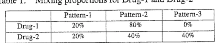
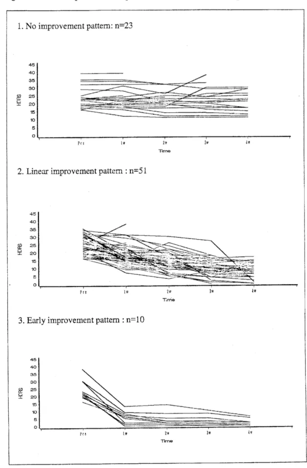
be grouped into the three patterns

shown in Figure 1. In Pattern-l, pretreatment

scores

are

maintained. This pattern corresponds to non-responders. Pattem-2 and Pattem-3 correspond to responders. In

Pattern-2,HDRS scoresdecrease almost Iinearlv. InPattern-3,the

scores

decrease

more

rapidly. The patient population

can

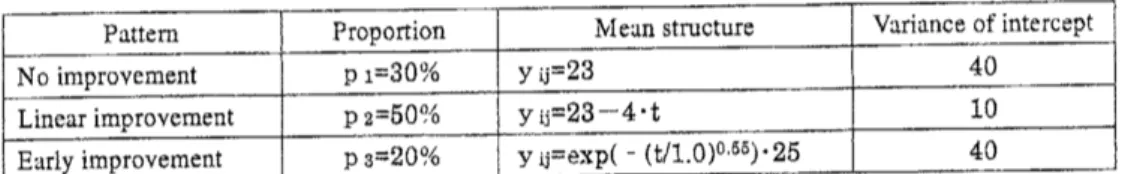
be considered as amixture of patients with the three

patterns. We here

suppose

two drugs, Drug-l and Drug-2, for which the mixing

proportionsof the three pattems

are

listedinTable 1.

Table 1. Mixingproportions for Drug-l andDrug-2

If the evaluation is made based only on the

mean

of the decrease at the final measurement point, the proportion of responders is 80% _{in either drug.} However, 40%

of the patients in Drug-2 show Pattem-3 and respond

more

rapidly. It is clear that Drug-2 is clinically more preferable. Such

an

evaluation can not be made if the

longitudinal patterns of HDRS

scores are

not considered. The efficacy of

antidepressants should be evaluatedbasedonthe longitudinalpatternsofHDRS

scores.

We apply mixture modelsto actual clinicaldata ofHDRS

scores.

We

assume

the

following three pattem $\mathrm{s}$ for the longitudinal patterns of HDRS scores, 1. No

improvementpattern,2. Linear improvementpattern,and 3.Early improvementpattem. In applying mixture models, it is

common

to

assume

that longitudinal patterns can be described by low-degree polynomials of elapsed time after the beginning of

treatment [16-19]. However, the low-degree polynomial models

are

not necessarily

appropriate for describing the longitudinal patterns ofHDRS

scores.

In Chapter 3 We propose

a

model using

a

monotone decreasing function to describe the early

(3)

187

improvement pattem. Furthermore, $\mathrm{V}\mathrm{Y}^{7}\mathrm{e}$ investigate variance-covariance structures

within a subject. In Chapter 4, YVe conduct simulation studies to evaluate the

performance of the proposed model in Chapter 3. In the chapter of discussion, YVe arrange the resultin this study. We derive the conclusion by present. And YVe refer the

problemof theproposedmethod and theviewofthe future.

MOTIVATING EXAMPLE

The present data

are

HDRS

scores

of

84

patients in

a

randomized, double-blind,

comparative study of antidepressants. Thecriteria for selecting the subjects

are

that the

total

score

forHDRS items 1-17

was

16 or

higher and thedepressive mood

score

of

was

$\underline{0}$orhigher,beforethe start of the treatment. Theantidepressants

were

given for4weeks,

following a fixed-flexible regimen. _The _{main item} ofevaluation

was

the final general improvement rating (FGIR) $\mathrm{e}\backslash _{t}$aluated by the physicians, taking into account the

changes in the HDRS

scores

and the clinical symptoms. FGIR

was

classified into eight

categories, $\mathrm{i}.\mathrm{e}.$, significant improvement, moderateimprovement, mild improvement,

no

change, slight worsening, worsening, serious worsening andimpossible to evaluate. The

HDRS

scores

were

evaluated at five measurement points, i.e., before the treatment and

1, 2, 3 and 4 weeks after the beginning of the treatment. The individual and mean profiles of HDRS

scores are

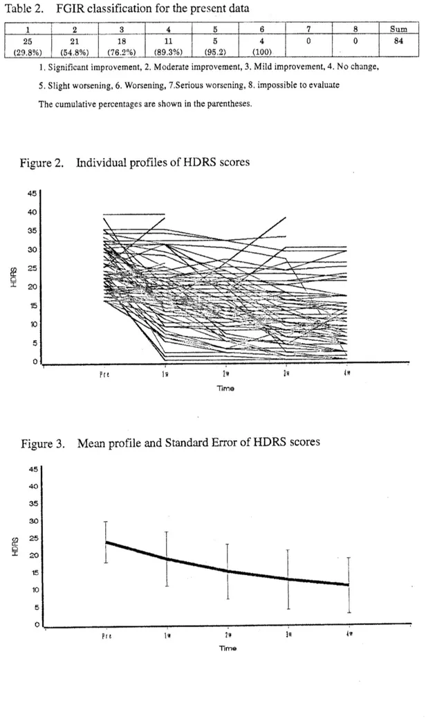
shown in Figure 2 and Figure 3, respectively. FGIR classificationfor thepresent datais shown inTable2.

(4)

(5)

189

Table 2. FGIR classificationforthepresentdata

1.Significantimprovement, 2.Moderateimprovement,3.Mild improvement,4,Nochange,

5. Slight worsening, 6.Worsening,7 Serious worsening,S.impossibletoevaluate

The cumulative percentagesareshowninthe parentheses.

Figure2. Individual profiles of HDRS

scores

TIrne

Figure 3. Mean profile and Standard ErrorofHDRS

scores

$[mathring]_{\ddagger \mathrm{Z}}\mathrm{a}\mathrm{e}$

(6)

190

MIXTURE DISTRIBUTIONMODELFOR

LONGITUDINAL

DATA

Mixture distribution models are often applied to the analysis of longitudinal

pattems ofrepeated measurements [16-19].

In this chapter, mixture distribution models

are

applied to HDRS

score

data

obtainedin

an

actual clinical trial of antidepressants.

(1) The model

As stated in the first chapter, longitudinal patterns of HDRS

scores

after the

administration of antidepressants

are

grouped into three patterns. We define the three

patterns asfollows.

1. No improvement pattern: the

scores

show no improvement maintaining the

pretreatment

scores.

2. Linear improvementpattern: the

scores

show almost linearimprovem $\mathrm{e}\mathrm{n}\mathrm{t}$.

3. Earlyimprovementpattern: the

scores

showrapid improvement.

These th $\mathrm{e}^{\alpha}$

.

patter $\mathrm{s}$ correspond to the three patterns shown in Figure 1. All of the

subjectsxe assumed tobelong to

one

ofthe $\mathrm{t}\mathrm{h}\mathrm{r}\mathrm{e}^{\Delta}$

.

patter $\mathrm{s}$.

Let yij denote the HDRS

score

of the patient $\mathrm{i}(\mathrm{i}=1,\cdots, \mathrm{n})$ at the measurement

point$\mathrm{t}_{\mathrm{j}}$ $(\mathrm{i}=1,\cdots, 5)$. In themixture distribution model, the probability density function

of the observation vector$\mathrm{y}_{\mathrm{i}}=(\mathrm{y}_{\mathrm{i}1},\cdots, \mathrm{y}_{\mathrm{i}5})$ isgiven by

$g$

(

$\mathrm{y}_{\mathrm{i}}$ I

$\mathrm{p},8$

)

$= \sum_{m=1}^{3}p_{m}\cdot f_{m}$($\mathrm{y}_{\mathrm{i}}$ I$8_{m}$), (1)

where $\mathrm{y}_{i}=(\mathrm{y}_{\mathrm{i}1},\mathrm{y}_{\mathrm{i}2},\mathrm{y}_{13},\mathrm{y}_{\mathrm{i}4},\mathrm{y}_{\mathrm{i}5})^{\mathrm{f}}$ is the measurement vector for the patient

$\mathrm{i}$, $\mathrm{p}=(\mathrm{p}_{1}, \mathrm{p}_{\underline{\gamma}}, \mathrm{p}_{3})$ $(\mathrm{p}_{1}+\mathrm{p}_{-}’\lrcorner_{-}\mathrm{p}_{3}=1)$ isthe vector ofthe mixingproportions ofthethree patterns,$f_{m}$ (

$\cdot$ ) is the

densityfunction forthe m-thpattern$(\mathrm{m}=1,2,3)$, $\mathrm{e}_{\mathrm{m}}$is the vector of theparameters that

defmethe densityfunction$f_{\mathfrak{l}n}$ $($

.

$)$ $(\mathrm{m}=1,2, 3)$,

$\mathrm{e}$ $=(8_{1}^{\mathrm{t}}, 8_{2}, {}^{\mathrm{t}}\mathrm{e}_{3}^{\mathrm{t}})^{\mathrm{t}}$denotes the vector of

all the parametersin $6_{1},6_{2}$ and

63.

For the threelongitudinal pattem $\mathrm{s}$statedabove,We

assume

thefollowing model.

1. No improvementpattem

(7)

I

E1

I

$L’)$. Linear improvementpattern

$\mathrm{y}_{ij}=(\alpha_{-},+\mathrm{b}_{2\mathrm{i}})+\beta_{2}\cdot \mathrm{t}+\epsilon_{\mathrm{o}_{1}}\mathrm{i}\sim \mathrm{J}$

3.

Earlyimprovementpattem

$y_{ij}=\exp(-(\mathrm{t}_{\mathrm{j}}/\alpha_{3})^{\beta_{\mathrm{j}}})\cdot(\gamma_{3}+\mathrm{b}_{3\mathrm{i}})+\epsilon_{3\mathrm{i}\mathrm{j}}$ ,

Inthis model, it is assumed thatthe pretreatment

scores

a1, a2, and$\mathrm{a}_{3}$

are

common

to all

thepatients ,$\mathrm{b}_{1\mathrm{i}}$, $\mathrm{b}\underline{\circ}\mathrm{i}$ and$\mathrm{b}_{3\mathrm{i}}$

are

thepatient-specific variations of the pretreatment

scores

normallydistributed

as

$\mathrm{b}_{1\mathrm{i}}\sim \mathrm{N}(0, \mathrm{s}_{\mathrm{b}12})$, $\mathrm{b}_{-:},\sim \mathrm{N}(0, \mathrm{s}\mathrm{b}22)$ and$\mathrm{b}_{3\mathrm{i}}\sim \mathrm{N}(0, \mathrm{s}\mathrm{b}22)$,respectivelyand

eiij, $\mathrm{e}_{2\mathrm{i}\mathrm{j}}$ and $\mathrm{s}3\mathrm{i}\mathrm{j}$ is the error term normally distributed with

mean

0 and

variance-covariance matrix $\Sigma_{\mathrm{s}1},\Sigma_{\epsilon^{\underline{\gamma}}}$ and $\Sigma_{\mathrm{s}3}$, respectively. The function of early

improvementpattern

comes

from the following:

1–(theWeibulldistributionfunction)$=1-(1-\exp(-(t/\alpha_{3})^{\beta_{3}}))=\exp(-(t/\alpha_{3})^{\beta_{3}})$,

This function is parsimonious and useful for describing monotone decreasing function.

In addition, this function

can

beused for describing thefeature ofHDRSpattern that the

variance for the early improvement pattern becomes smaller

as

the clinical trial

advances. Thedetailsaregivenlater.

(2) The

variance-covariance

within apatient

For the

variance-covariance

matrices of the

error

terms, the following three

struc

rures

are employed: simple variance (SV), first-order autoregressive $(\mathrm{A}\mathrm{R}(1))$, and

toeplitz (TOEP), which are commonlyused in the analysis ofclinical longitudinal data

[20].

When SV is assumed, the

variance-covariance

matrix of the marginal distribution becomes a compound symmetry type in the no improvement pattern and

linearimprovementpattemasfollows:

$\ovalbox{\tt\small REJECT}_{1}^{1}1\ovalbox{\tt\small REJECT} 11^{\cdot}[\sigma_{bm}^{2}]\cdot[1 1 1 1 1]+\{$$\sigma_{\epsilon_{0}0^{m}}^{2}00$

$\sigma_{m}^{2}0000$ $\sigma_{m}^{2}0000$ $\sigma_{m}^{2}0000$ $\sigma_{\epsilon m}000\ovalbox{\tt\small REJECT} 0_{2}$

,$\mathrm{m}=1,2$.

(8)

1 EI2

$\ovalbox{\tt\small REJECT}_{\exp(}^{\exp(}\exp\{\exp\langle\exp\langle-\langle 4/\alpha_{3})^{\beta_{3}})-(2/\mathrm{a}_{3})^{p_{3}})-(0/\alpha_{3})^{\beta\underline{\tau}})-(3/\alpha_{3}\}^{\beta 3})-(1/\alpha 3)^{\beta 3})\ovalbox{\tt\small REJECT}$ .

$[_{\sigma_{b3}}2]\ovalbox{\tt\small REJECT}_{\exp\{}^{\exp(}\mathrm{e}\mathrm{x}.\mathrm{p}(\exp(\exp(-(2/\alpha_{3}\rangle^{\beta 3})\ovalbox{\tt\small REJECT}^{t}\wedge(0/\alpha_{3}\rangle^{\beta 3})-(4/\mathrm{a}_{3}\}^{\beta_{3}})-(3/\alpha_{3})^{\beta_{3}})-(1/\alpha_{3})^{\beta 3})+\ovalbox{\tt\small REJECT}$

a

$\epsilon_{0}30002$ $\sigma_{\mathrm{s}_{0}3}000_{\wedge}$

”

$\sigma_{\epsilon_{0}3}0\mathrm{o}_{\wedge}\mathrm{o}_{9}$ $\sigma_{\epsilon_{0}3}0_{2}00$ $\sigma\epsilon 300\ovalbox{\tt\small REJECT} 002$

From this structure, it is found that the variance becomes smaller

as

the clinical trial

advances and that the covariance becomes smaller as the interval between the

measurement points becomes longer.

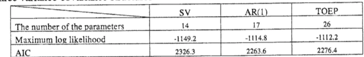
(3) Results

Table 3 shows the number of theparameters, maximum $10^{\sigma}\underline{\sim}$likelihood andAIC

[21-23] for the three variance-covariance structures, $\mathrm{S}\mathrm{V}$, $\mathrm{A}\mathrm{R}(1)$,

or

TOER The AICs

indicate that the

variance-covariance

structure $\mathrm{A}\mathrm{R}(1)$ is the best

among

the three

structures.

Table

3.

Thenumberofthe parameters, maximum$\log$ likelihoodandAICfor the

The result when $\mathrm{A}\mathrm{R}(1)$ is assumed is shown

as

follows. Table 4 lists the

maximum likelihood estimates of the parameters and their standard

errors.

Figure 4

(9)

163

Table4. Themaximumlikelihood estimates(MLE) and theirstandard

errors

Pattem Parameter MLE $\mathrm{S}.\mathrm{E}$.

$\mathrm{p}1$ 0.298 0.030

$\alpha 1$ 22.4 1.762

1. Noimprovementpattem $\sigma$

$\mathrm{b}$$12$ 8.43 2.639 $\sigma$ $p$ $12$ 40.4 2.349 $p1$ 0.875 o.oos $\mathrm{p}2$ 0.581 0.122 $a\mathrm{z}$ 23.4 0.818

2. Linear improvementpattern

$\mathcal{B}\mathrm{r}$ -4.0 0.285

$\sigma$$\mathrm{b}2^{2}$

o.oo

3.847

$\sigma$ $\epsilon$ $2^{2}$ 33.6 3893 $\beta 2$ 0.553 0.066 $\mathrm{p}$a 0.121 $\alpha_{\mathit{3}}$ 0.283 0.053

3. Early improvement pattern

$\beta_{3}$ 0.309 0.070 $\gamma s$ 23.5 3.554 $\sigma$$\mathrm{b}3^{2}$ 31.9 9 $6\hat{0}6$ $\sigma$ $P$ $3^{2}$ 11.5 0477 $\rho s$ 0.859 0.011

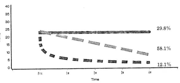
Figure4. Theestimated

mean

profiles of HDRS

scores

for the three pattem $\mathrm{s}$

$[mathring]_{\mathrm{x}}\not\in$

(10)

194

Given the estimatesfor all the parameters, the probabilities that the patient $\mathrm{i}$ with

the data $\mathrm{y}_{\mathrm{i}}$belongs to each of the three patterns

can

be estimated by Bayes theorem

[24-26]. By assuming that each patientbelongs to the pattern forwhich the probability

is the largest, thepatientscanbeclassifiedintothethree patterns. Theproportions of the

patients classified into the three patterns are 27.4%(23/84: No improvement), 60.7% (51/84: Linear improvement) and 11.9% (10/84: Early improvement). The relationship

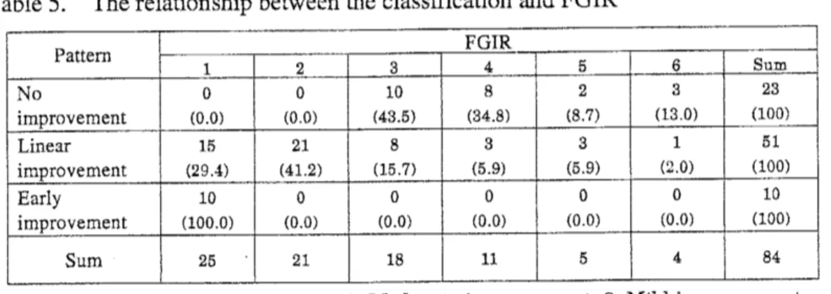
between theclassification andFGIR measured in the clinicaltrial is shown in Table 5.

Figure 5 shows theindividual profiles ofthepatientsclassified intothe three patterns.

Table

5.

Therelationshipbetween theclassification and FGIR

4.No change,5. Slight worsening,6.Worsening

(11)

185

(12)

198

From the results assuming the variance-covariance structure $\mathrm{A}\mathrm{R}(1)$, the following

points

can

befound

1. The estimated pretreatment

scores are

22.4,

23.4

and 23.5 for the no

improvementpattern, linear improvementpattern and earlyimprovementpattem,

respectively. There

seems

tobeno greatdifferencesamongthe three patterns.

$\mathrm{i}\mathrm{i}$

.

The estimated mixing proportions

are

29.8%, 58.1%, and 12.1% for the no

improvementpattern, linear improvementpattem, andearly improvement pattem, respectively. About 70% of the patientsbelong to eitherthe linearimprovement

pattern

or

earlyimprovementpattern.

$\ddot{\dot{\mathrm{m}}}$. The estimated

scores

at 1 week after thebeginning of the treatment

are 19.4

and

5.4 in the linear improvement pattern and early improvement pattern,

respectively. The estimated

scores

at 2 weeks

are

15,4 _and 3.8 in the linear

improvement pattern and early improvement pattem, respectively. The results

suggest that the HDRS

scores

had been improved clinically well enough at 1

week in theearlyimprovementpattern.

$\mathrm{i}\mathrm{v}$

.

The estimated

scores

atthe final measurementpoint(4weeksafter thebeginning

of the treatment)

are

22.4,

7.4

and 2.4 in the

no

improvement pattern, linear

improvement pattern and early improvement pattern, respectively. The HDRS

scores were

improvedinboth the linear andearly improvementpatterns.

$\mathrm{v}$. The estimated probabilities that each patient belong to each ofthe three patients

rangefrom

0.504

to 1.000 with

mean 0.892.

25,

50

and75 percentiles

are

0.836,

0.966

and0.998,respectively.

$\mathrm{v}\mathrm{i}$

.

Theproportionsof thepatients classified into the three patterns

are

27,4% (23/84),

60.7% (51/84), and 11.9% (10/84) for the

no

improvement pattem, linear

improvement pattem, and early improvement pattern, respectively. These

are

almostthe

same as

theestimatesof themixing proportion.

$\mathrm{V}\vec{11}$

.

The relationship between the results of the classificationand FGIR indicates that

all the patients classified into the early improvement pattern showed the significant improvement in FGIR and that about

85

% of the patients classified into the linear improvement pattern showed the mild

or

better improvement in FGIR. On the otherhand, thepatientsclassified intothe

no

improvement pattern

(13)

1S7

did not show themoderate

or

betterimprovementin FGIR.

SIMULATION

STUDY:DETECTION

OF TRUE VA RIANCE-COVARIANCE

STRUCTURE

When repeated measurements of HDRS

scores are

analyzed using the mixture distribution model consisting ofthe three patterns (no improvement, linear improvement,

andearlyimprovement)presented in Chapter3, it is importantto examine the influence of the assumption of the within-subject covariance structure on the parameter estimates. In this chapter,the following two simulation studies

are

conductedtoexamine thisissue.

Inthe simulation study, We suppose the situation inwhich themodel with thetrue

within-subjectcovariance structureis includedin the appliedmodels. Under this situation,

it is examined whether the selected model

can

detect the true structure of the

within-subject covariance. In addition, We examine the influence of the mis-specified

within-subjectcovariancestructure

on

the accuracyof the parameterestimates.

In this simulation study, thefollowing three structures, $\mathrm{S}\mathrm{Y}$,

$\mathrm{A}\mathrm{R}(1)$, and TOEP are

assumed for the within-subject covariance structure. T.a$\mathrm{b}\mathrm{l}\mathrm{e}$ $6$ shows the true values of the

parameters. Thesevalues

are

determinedby referring to theresultsin Chaper3.

Underthe true structure, 100 data sets

are

simulated. Each data setconsistsof the

data of 100 subjects. For each data set, the three mixture distribution models with the

within-subject covariance structure$\mathrm{S}\mathrm{V}$,$\mathrm{A}\mathrm{R}(1)$, and TOEP

are

appliedand the goodness of

each model isevaluatedbased

on

theAIC[21-23].

Table 7 shows the proportions that each mixture distribution model is selected based

on

AIC. The proportion that the true within-subject covariance structure model is selected is about95% for each of the three within-subjectcovariance structure. Thisresult

suggests thattheproposed approach

can

selectthe truewithin-subjectcovariance structure

underthe situation in which the modelwith the true within-subject covariance structureis

includedinthe appliedmodels.

The description of the result is omitted, and the following is confirmed. The

accuracy of the estimates is especially worsened for the following

cases:

SV is assumed

when the true structure is $\mathrm{A}\mathrm{R}$, and SV

or

$\mathrm{A}\mathrm{R}(1)$ is assumed when the true structure is

(14)

198

(15)

199

DISCUSSION

It is problem from clinical viewpoints that the efficacy of antidepressant is evaluated based

on

the

mean

ofthe decrease of HDRS

scores

at the final measurement point, becausethe longitudinal$\mathrm{p}\mathrm{a}\mathrm{t}\mathrm{t}\frac{-}{}.\mathrm{m}$ofHDRS

scores

of eachpatient isnotconsidered.

In thepresent study,

we

have evaluated the results on thebasis of$1\mathrm{o}\mathrm{n}_{arrow}\sigma$-itudinalpatterns.

Byevaluating the averagechanges ineach pattern and the $\mathrm{m}\dot{\mathrm{L}}\mathrm{X}\mathrm{i}\mathrm{n}_{\underline{arrow}}\sigma$proportions, we could

quantitatively evaluate the early onset of

a

characteristic feature of the drug. The

analyses at each time point cause the statistical problem ofmultiplicity, and the results

are

difficulttounderstand. Because theobjective ofthe analyses ateachtimepoint isto

evaluate

on

the longitudinal patterns,the evaluationispossibleby thismethod.

The results ofthis study and the clinical evaluation (FGIR) of the subjects have

acertain level ofagreement. Therefore,

we can

conclude that this method isappropriate

from theclinical pointofview. Theresults suggest that FGIR isan evaluation inwhich

longitudinalpatterns

are

takeninto account. By classifying the subjects into

one

of the

three patterns,

we can

examine the differences in background factors among subjects

having these differentpattems.

By applying thismethod, itis possible to execute comparisonbetween drugs by themixtureproportions of the drug. Thenullhypothesis ofcomparisonbetween Drug-l andDrug-2 _inthiscaseisasfollows.

$\mathrm{H}_{0\mathrm{P}\mathrm{m},\mathrm{D}\sigma- 1^{=\mathrm{p}_{\mathrm{m},\mathrm{I}\supset \mathrm{r}\mathrm{u}\mathrm{g}-\underline{0}}}}:\mathrm{r}\mathrm{u}_{\mathrm{s}}$ : $\mathrm{m}=1,2,3$,

where$\mathrm{p}_{\mathrm{m}}$ismixingproportionof m-th pattern.

This partwillneed examining inthe future.

One problem with this methodis how to decide

on

the number ofpatterns to be

used. This has not been solved in the present study. In this study, the analysis is done

assuming 3 patterns, taking into account the observed data and

an

easiness of clinical

explanation. When the number of patterns is decided,

we

should decide it in considerationof

a

feature ofthe drug andaclinical meaning.

In the analysis ofthis study,

we

assumed that all the subjects belonged to

one

of

the three variation pattem $\mathrm{s}$. It is quite possible that data of

some

subjects may be

intermediate between twopatterns in fact. Areas tobe studied in the future include the

(16)

200

The variance-covariance structure within a patient is actually unknown. It is

necess

ary to investigate the influence of misspecification the

variance-covariance

structure within a patient. In actual analyses, it is quite difficult to specify the correct

variance-covariance

structure within

a

subject. It will be desirable to

use

a robust

estimationmethod against the $\mathrm{m}\mathrm{i}\mathrm{s}$-specification cf

variance-covariance

structure within

asubject.

REFERENCES

1. Bech P. A meta-analysis of the antidepressant properties of serotonin reuptake

inhibitors.International Review ofPsychiatry 1990; 2: 207-211

2. Sitsen$\mathrm{J}_{1}^{\backslash }\cdot \mathrm{I}\mathrm{A}$, ZivkovM. Mirtazapine Clinical Profile. CNS Drugs 1995;$4(1)$:

39-48

3. Grimsley SR, Jann MW Drug Reviews: Paroxetine, sertraline and fluvoxamine:

New selective serotoninreuptake inhibitors. ClinicalPharmacy 1992; 11:930-957 4. Kasper S, Fuger J, Moller HI Comparative Efficacy of Antidepressants. Drugs

1992;43(2): 11-23

5. DavisJM, Wang Z, Janicak PG A Quantitative Analysis ofClinicalDrug Trialsfor

the Treatment of Affective Disorders. Psychopharmacology Bulletin

1993

;29(2):

175-181

6. Anderson $\mathrm{I}\mathrm{M}_{\sim}$ Tomenson BM. Treatment discontinuation with selective serotonin

reuptake inhibitors comared with tricyclic antidepressants:

a

meta-analysis BMJ

1995; 310(3):

14334438

7. MontgomerySA,Kasper S. Comparisonofcompliancebetween serotonin reuptake

inhibitors and tricyclic antidepressants:

a

meta-analysis. International Clinical

Psychopharmacology 1995;$9(4)$: 33-40

8. Moller HJ, VolzHP. Drug Treatment ofDepression in the

1990s.

Drugs 1996;

52:

625-638

9.

AnsseauM,PapartP, Troisfontaines B, etal. Controlled comparison of milnacipran

andfluoxetine in major depression. Psychopharmacology 1994; 114: 131-137

10.

Remick RA, Reesal R, Oakander M, et al. Comparison of FLUVOXAMINE and

AMITRIPTY LINE in depressed outpatients. Cument Therapeutic Research 1994;

55(3):

243-250

11. Artigas F. Selective $\mathrm{S}\mathrm{e}\mathrm{r}\mathrm{o}\mathrm{t}\mathrm{o}\mathrm{n}\mathrm{i}\mathrm{n}/$ Noradrenaline Reuptake Inhibitors(SNRIs)

Pharmacology andTherapeutic Potentialin the Treatment of Depressive Disorders. CNS Drugs 1995;$4(2)$

: 79-89

(17)

201

reuptake inhibitors in major depression. International Clinical Psychophamacology

1996; 11(4): 41-46

13. Hamilton M. A rating scale for depression. J.Neurol.Neurosurg.Psychiat 1960; 23: 56-62

14. Hamilton M. Development of a rating scale for primary depressive illness. Brit.

soc.

din. Psychol 1967; 6:

278-296

15. WilliamsJBW.Arch GenPsychiatry 1988;45: 742-747

16. Tango T. A mixturemodeltoclassifyindividualprofilesofrepeated measurements. Data science: classification andrelatedmethods 1998; 247-254

17. Tango T. Mixture models for the analysis of repeated measurements in clinical

traials. JapaneseJournal Applied Statistics 1989; 18: 143-161

18. Skene AM,WhiteSA. Alatent classmodel forrepeatedmeasurements experiments. Statist. Med.1992; 11:2111-2122

19. Pavlic M, Brand RJ, Cummings SR. Estimating probability of

non-response

to

beatmentusing_mixture

_{distributions.}

Statist. Med. 2001; 20:

1739-1753

20.

Verbeke G, Molenberghs G. Linear Mixed Models for Longitudinal Data;

2000:

Springer

21. Akaike H. hfomation theory and an extension of the maximum likelihood principle, $2^{\mathrm{n}\mathrm{d}}$ International Symposium on Information Theory. Akademiai Kiado,

Budapest 1973;