Evolutes and involutes of fronts in the Euclidean plane (Pursuit of the Essence of Singularity Theory)

Evolutes

and

involutes

of fronts

in

the

Euclidean

plane

Masatomo Takahashi,

Muroran Institute of Tecnhology Abstract

This is a survey on evolutes and involutes of curves in the

Eu-clidean plane. The evolutes and the involutes for regular curves are

the classical object. Even if a curve is regular, the evolute and the

involute of the curve mayhave singularities. By using a moving frame

of the front and the curvature of the Legendre immersion, we define

an evolute and an involute of the front (the Legendre immersion in

the unit tangent bundle) in the Euclidean plane anddiscuss properties

of _{them. We also consider about relationship between evolutes and}

involutesoffronts. Wecan observe that the evolutes andthe involutes

offronts are corresponding to the differential and integral in classical

calculus.

1

Introduction

The notions ofevolutes and involutes (also known as evolvents) have studied

by C. Huygens in his work [13] and they have studied in classical analysis,

differential geometry and singularity theory of planar

curves

(cf. [3, 8, 10,

11, 19, 20]$)$. The evolute of a regular

curve

in the Euclidean

plane is given

by not only the locus of all its centres of the curvature (the caustics of the

regular curve), but also the envelope of normal lines of the regular curve,

namely, the locus of singular loci of parallel

_curves

(the

wave

front of the

regular curve). On the other hand, the involute of

a

regular

curve

is the trajectory $d\dot{e}$scribed by the end of stretched

string unwinding from

a

point

of the

curve.

Alternatively, another way to construct the involute of

a

curve

is to replace the taut string by a line segment that is tangent to the

curve

on one

end, while the other end traces out _{the involute. The length of the}

line segment is changed by

an

amount equal to the

arc

length traversed by

the tangent point

as

it

moves

along the

curve.

In \S 2,

we

give a brief review on the theory of regular curves, define the classical evolutes and involutes. It is well-known that the relationship

be-tween evolutes and involutes of regular plane

curves.

In \S 3, we consider

give the curvature of the Legendre

curve

(cf. [5]). We give the existence

and the uniqueness Theorems for Legendre

curves

like

as

regular

curves.

By

using the curvature of the Legendre immersion,

we

define evolutes and

in-volutes of fronts in

\S 4

and

\S 5

respectively. We

see

that the evolute of the front is not only $a$ (wave) front but also

a

caustic in

\S 4.

Moreover, the

in-volute of the front is not only $a$ (wave) front but also

a

caustic in

\S 5.

The

study of singularities of (wave) fronts and caustics is the starting point of

the theory of Legendrian and Lagrangian singularities developed by several

mathematicians and physicists $[$1, 2, 4, 9, 12, 15, 16, 17, 18, 21, 22, 23, $24]$ etc.

Furthermore,

we can

observe that the evolutes and the involutes offronts

are

corresponding to the differential and integral in classical calculus in

\S 6.

This is the announcement of results obtained in [5, 6, 7]. Refer [5, 6, 7]

for detailed proofs, further properties and examples.

We shall

assume

throughout the whole paper that all maps and manifolds

are $C^{\infty}$ unless the contrary is explicitly stated.

Acknowledgement. We would like to thank Professors Takashi Nishimura

and Kentaro Saji for holding of the workshop. The author

was

supported by

a

Grant-in-Aid for Young Scientists (B) No.

23740041.

2

Regular plane

curves

Let $I$ be an interval

or

$\mathbb{R}$. Suppose that

$\gamma$ :

$Iarrow \mathbb{R}^{2}$ is

a

regular plane curve,

that is, $\dot{\gamma}(t)\neq 0$ for any $t\in I$

.

If $s$ is the arc-length parameter of $\gamma$,

we

denote $t(s)$ by the unit tangent vector $t(s)=\gamma’(s)=(d\gamma/ds)(s)$ and $n(s)$

by the unit normal vector$n(s)=J(t(s))$ of$\gamma(s)$, where $J$is the anticlockwise

rotation by $\pi/2$. Then we have the Frenet formula

as

follows:

$(\begin{array}{l}t’(s)n’(s)\end{array})=(\begin{array}{ll}0 \kappa(s)-\kappa(s) 0\end{array})(\begin{array}{l}t(s)n(s)\end{array}),$

where

$\kappa(s)=t’(s)\cdot n(s)=\det(\gamma’(s), \gamma"(\mathcal{S}))$

is the curvature of$\gamma$ and is the inner product

on

$\mathbb{R}^{2}.$

Even if$t$ is not the arc-length parameter,

we

have the unit tangent vector

$t(t)=\dot{\gamma}(t)/|\dot{\gamma}(t)|$, the unit normal vector $n(t)=J(t(t))$ and the Frenet

formula

where $\dot{\gamma}(t)=(d\gamma/dt)(t),$ $|\dot{\gamma}(t)|=\sqrt{\gamma(t)\gamma(t)}$ and the curvature is given by

$\kappa(t)=\frac{i(t)\cdot n(t)}{|\dot{\gamma}(t)|}=\frac{\det(\dot{\gamma}(t),\ddot{\gamma}(t))}{|\dot{\gamma}(t)|^{3}}.$

Note that the curvature $\kappa(t)$ is independent

on

the choice of

a

parametrisa-tion.

Let $\gamma$ and $\tilde{\gamma}$ : $Iarrow \mathbb{R}^{2}$ be regular

curves.

We say that

$\gamma$ and

$\tilde{\gamma}$

are

congruent if there exists

a

congruence

$C$

on

$\mathbb{R}^{2}$ such that

$\tilde{\gamma}(t)=C(\gamma(t))$

for all $t\in I$, where the congruence $C$ is

a

composition of

a

rotation and

a

translation

on

$\mathbb{R}^{2}.$

As well-known results, the existence and the uniqueness for regular plane

curves

are as

follows (cf. [8, 10]):

Theorem 2.1 (The Existence Theorem) Let $\kappa$ : $Iarrow \mathbb{R}$ be

a

smooth

func-tion. There exists a regular parametrised

curve

$\gamma$ :

$Iarrow \mathbb{R}^{2}who\mathcal{S}e$ associated

curvature

_function

is $\kappa.$

Theorem 2.2 (The Uniqueness Theorem) Let $\gamma$ and

$\tilde{\gamma}$ : $Iarrow \mathbb{R}^{2}$ be regular

curves

whose speeds $s=|\dot{\gamma}(t)|$ and $\tilde{s}=|\tilde{\gamma}(t)|$, and also curvatures $\kappa$ and X

each coincide. Then $\gamma$ and $\tilde{\gamma}$

are

congruent.

In fact, the regular

curve

whose associated curvature function is $\kappa$, is

given by the form

$\gamma(t)=(\int\cos(\int\kappa(t)dt)dt, \int\sin(\int\kappa(t)dt)dt)$

In this paper,

we

consider evolutes and involutes of plane

_curves.

The

evolute $Ev(\gamma)$ : $Iarrow \mathbb{R}^{2}$

of

a regular plane

curve

$\gamma$ :

$Iarrow \mathbb{R}^{2}$ is given by

$Ev( \gamma)(t)=\gamma(t)+\frac{1}{\kappa(t)}n(t)$, (1)

away from the point $\kappa(t)=0$, i.e., without inflection points (cf. [3, 8, 10]).

On the other hand, the involute $Inv(\gamma, t_{0})$ : $Iarrow \mathbb{R}^{2}$

of

a

regular plane

curve $\gamma$ : $Iarrow \mathbb{R}^{2}$ at $t_{0}\in I$ is given by

$Inv( \gamma, t_{0})(t)=\gamma(t)-(\int_{t_{0}}^{t}|\dot{\gamma}(s)|ds)t(t)$. (2)

Example 2.3 (1) Let $\gamma$ : $[0,2\pi)arrow \mathbb{R}^{2}$ be

an

ellipse $\gamma(t)=((x\cos t, b\sin t)$

with $a\neq b$. Then the evolute of the ellipse is

The evolute of the ellipse with $a=3/2,$$b=1$ is pictured

as

Figure lleft.

(2) Let $\gamma$ : $[0,2\pi)arrow \mathbb{R}^{2}$ be a circle $\gamma(t)=(r\cos t, r\sin t)$. Then the

involute of the circle at $t_{0}$ is

$Inv(\gamma, t_{0})(t)=(r\cos t-r(t-t_{0})\sin t, r\sin t+r(t-t_{0})\cos t)$.

The involute of the circle with $r=1$ at $t_{0}=\pi$ is pictured

as

Figure 1 right.

-.

(1) the evolute of

an

ellipse (2) the involute of

a

circle at $\pi$

Figure 1.

The following properties

are

also well-known in the classical differential

ge-ometry of

curves:

Proposition 2.4 Let $\gamma$ :

$Iarrow \mathbb{R}^{2}$ be a regular

curue

and _{$t_{0}\in I.$}

(1)

_If

$t$ is

a

regular point

of

$Inv(\gamma, t_{0})$, then $Ev(Inv(\gamma, t_{0}))(t)=\gamma(t)$.

(2) Suppose that $t_{0}$ is

a

regular point

of

$Ev(\gamma)$

.

If

$t$ is

a

regular point

of

$Ev(\gamma)$, then $Inv(Ev(\gamma), t_{0})(t)=\gamma(t)-(1/\kappa(t_{0}))n(t)$.

Note that

even

if $\gamma$ is

a

regular curve, $Ev(\gamma)$ may have singularities and

also $t_{0}$ is

a

singular point of $Inv(\gamma, t_{0})$,

see

Figure 1. For

a

singular point of

$Ev(\gamma)$ $($respectively, $Inv(\gamma, t_{0})$), the involute $Inv(Ev(\gamma), t_{U})(t)$ (respectively,

the evolute $Ev(Inv(\gamma, t_{0}))(t))$

can

not deflne by the definition of the evolute

and the involute. In general, if $\gamma$ is not a regular curve, then we can not

define the evolute and the involute of the

curve.

In this paper, we define the evolutes and the involutes with singular

points,

_{see \S 4}

and

\S 5.

In order todescribe these definitions, we introduce the

notion of fronts in the next section.

3

Legendre

curves

and

Legendre

immersions

We say that $(\gamma, v)$ : $Iarrow \mathbb{R}^{2}\cross S^{1}$ is

a

Legendre

curve

if $(\gamma, v)^{*}\theta=0$ for

$\prime 1_{1}’\mathbb{R}^{2}=\mathbb{R}^{2}xS^{1}$ (cf. [1, 2]). This condition is equivalent

to $\dot{\gamma}(t)\cdot\nu(t)=0$

for all $t\in I$. Moreover, if $(\gamma, v)$ is an immersion,

we

call $(\gamma, v)$ a Legendre

immersion. We say that $\gamma$ :

$Iarrow \mathbb{R}^{2}$ is

a

frontal

(respectively, a

_front

or $a$

wave

front) if there exists

a

smooth mapping $v$ : $Iarrow S^{1}$ such that $(\gamma, v)$ is

a Legendre

curve

(respectively, a Legendre immersion).

Let $(\gamma, \nu)$ : $Iarrow \mathbb{R}^{2}\cross S^{1}$ be

a

Legendre

curve.

Then

we

have the Frenet

formula of the frontal $\gamma$ as follows. We put on $\mu(t)=J(\nu(t))$. We call the

pair $\{v(t), \mu(t)\}$

a

moving

frame of

the

frontal

$\gamma(t)$ in $\mathbb{R}^{2}$ and

the Frenet

formula of the frontal (or, the Legendre curve) which is given by

$(\begin{array}{l}\dot{v}(t)\dot{\mu}(t)\end{array})=(\begin{array}{ll}0 \ell(t)-l(t) 0\end{array})(\begin{array}{l}v(t)\mu(t)\end{array}),$

where $\ell(t)=\dot{\nu}(t)\cdot\mu(t)$. Moreover, if $\dot{\gamma}(t)=\alpha(t)v(t)+\beta(t)\mu(t)$ for

some

smooth $f\iota$mctions _$\alpha(t),$

$\beta(t)$, then $\alpha(t)=0$ follows from the condition $\dot{\gamma}(t)$ .

$\nu(t)=0$. Hence, there exists a smooth function $\beta(t)$ such that

$\dot{\gamma}(t)=\beta(t)\mu(t)$ .

The pair $(\ell, \beta)1s$

an

important invariant of Legendre

curves

(or, frontals).

We call the pair $(P(t), \beta(t))$ the curvature

of

the Legendre curve (with respect

to the parameter $t$).

Definition 3.1 Let $(\gamma, \nu)$ and $(\tilde{\gamma}, \tilde{v}):Iarrow \mathbb{R}^{2}\cross S^{1}$ be Legendre

curves.

We say that $(\gamma, v)$ and $(\tilde{\gamma}, \tilde{\nu})$ are congruent as Legendre

curves

if there exists

a

congruence $C$

on

$\mathbb{R}^{2}$ such that

$\tilde{\gamma}(t)=C(\gamma(t))=A(\gamma(t))+b$ and $\tilde{\nu}(t)=$

$A(v(t))$ for all $t\in I$, where $C$ is given by the rotation $A$ and the translation

$b$ on $\mathbb{R}^{2}.$

We have the existence and the uniqueness for Legendre

curves

in the unit

tangent bundle like

as

regular plane curves,

see

in [5].

Theorem 3.2 (The Existence Theorem) Let $(P, \beta)$ : $Iarrow \mathbb{R}^{2}$ be a smooth

mapping. There exists aLegendre

curve

$(\gamma, v)$ : $Iarrow \mathbb{R}^{2}\cross S^{1}$ whose associated

curvature

_of

the Legendre

curve

is $(\ell, \beta)$

.

Theorem 3.3 (The Uniqueness Theorem) Let $(\gamma, \nu)$ and $(\tilde{\gamma}, \tilde{v})$ : $Iarrow \mathbb{R}^{2}\cross$

$S^{1}$ be Legendre

curv

$e\mathcal{S}$ whose curvatures

of

Legendre

curves

$(P, \beta\} and (\tilde{\ell,}\tilde{\beta})$

coincide. Then $(\gamma, v)$ and $(\tilde{\gamma}, \tilde{v})$ are congruent as Legendre

curves.

curve

is $(\ell, \beta)$, is given by the form

$\gamma(t)$ $=$ $(- \int\beta(t)\sin(\int\ell(t)dt)dt,$ $\int\beta(t)\cos(\int I(t)dt)dt)$ ,

$v(t)$ $=$ $( \cos\int\ell(t)dt,$ $\sin\int\ell(t)dt)$

Remark 3.4 By definition of the Legendre curve, if $(\gamma, v)$ is

a

Legendre

curve, then $(\gamma, -v)$ is also. In this case, $\ell(t)$ does not change, but $\beta(t)$

changes $to-\beta(t)$

.

Let $I$ and $\overline{I}$ be intervals. _$A$ smooth,function $s:\overline{I}arrow I$ is

$a$ (positive) change

of

parameterwhen 9 is surjective and has

a

positive derivative at every point.

It follows that $s$ is

a

diffeomorphism map by calculus.

Let $(\gamma, \nu)$ : $Iarrow \mathbb{R}^{2}\cross S^{1}$ and $(\overline{\gamma},\overline{\nu})$ : $\overline{I}arrow \mathbb{R}^{2}\cross S^{1}$ be Legendre

curves

whose curvatures of the Legendre

curves are

$(\ell, \beta)$ and $(\overline{\ell}, \overline{\beta})$ respectively.

Suppose $(\gamma, v)$ and $(\overline{\gamma}, \overline{v})$

are

parametrically equivalent via the change of

parameter $s:\overline{I}arrow I$

.

Thus $(\overline{\gamma}(t),\overline{v}(t))=(\gamma(s(t)), \nu(s(t)))$ for all $t\in\overline{I}$. By

differentiation, we have

$\overline{\ell}(t)=\ell(s(t))_{\dot{6}}(t), \overline{\beta}(t)=\beta(s(t))\dot{s}(t)$.

Therefore, the curvature of the Legendre

curve

is depended

on a

parametri-sation. We give examples of Legendre

curves.

Example 3.5 One of the typical example of

a

front (and hence

a

frontal)

is

a

regular plane

curve.

Let $\gamma$ :

$Iarrow \mathbb{R}^{2}$ be

a

regular plane

curve.

In this

case,

we

may take $v:Iarrow S^{1}$ by _$v(t)=n(t)$. Then it is easy to check that

$(\gamma, \nu)$ : $Iarrow \mathbb{R}^{2}\cross S^{1}$ is

a

Legendre immersion (a Legendre curve).

By

a

direct calculation,

we

give

a

relationship between the curvature of the

Legendre

curve

$(\ell(t), \beta(t))$

and

the curvature $\kappa(t)$ if $\gamma$ is

a

regular

curve.

Proposition 3.6 ([6, Lemma3.1]) Under the above notions,

_if

$\gamma$ is a regular

curve, then $\ell(t)=|\beta(t)|\kappa(t)$.

Example 3.7 Let $n,$ $m$ and $k$ be natural

numbers

with $m=n+k$. Let

$(\gamma, v):Iarrow \mathbb{R}^{2}\cross S^{1}$ be

$\gamma(t)=(\frac{1}{r\iota}t^{n}, \frac{1}{rr\iota}t^{m}), v(t)=\frac{1}{\sqrt{t^{2k}+1}}(-t^{k}, 1)$ .

It is easy to

see

that $(\gamma, \nu)$ is

a

Legendre curve, and

a

Legendre immersion

(2, 3) has the 3/2 cusp ($A_{2}$ singularity) at $t=0$, of type (3, 4) has the

4/3 cusp ($E_{6}$ singularity) at $t=0$ and of type (2,5) has the 5/2 cusp $(A_{4}$

singularity) at $t=0$,

see

Figure 2 (cf. [2, 3, 14]). By definition,

we

have

$\mu(t)=(1/\sqrt{t^{2k}+1})(-1, -t^{k})$ and

$\ell(t)=\frac{kt^{k-1}}{t^{2k}+1}, \beta(t)=-t^{n-1}\sqrt{t^{2k}+1}.$

the 3/2 cusp the 4/3 cusp the 5/2 cusp

Figure 2.

More generally,

we see

that analytic

curves

$\gamma$ :

$Iarrow \mathbb{R}^{2}$

are

frontals.

Now, we consider Legendre immersions in the unit tangent bundle. Let

$(\gamma, \nu)$ : $Iarrow \mathbb{R}^{2}\cross S^{1}$ be

a

Legendre immersion. Then the curvature of the

Legendre immersion $(P(t), \beta(t))\neq(O, 0)$ for all $t\in I$. In this case, we define

the normalized curvature

_for

the Legendre immersion by

$( \overline{\ell}(t),\overline{\beta}(t))=(\frac{l(t)}{\sqrt{l(t)^{2}+\beta(t)^{2}}}\frac{\beta(t)}{\sqrt{l(t)^{2}+\beta(t)^{2}}})$

Then the normalized curvature $(\overline{\ell}(t), \overline{\beta}(t))$ is independent on the choice of

a

parametrisation. Moreover, since $\overline{l}(t)^{2}+\overline{\beta}(t)^{2}=1$, there exists

a

smooth

function $\theta(t)$ such that

$\overline{l}(t)=\cos\theta(t), \overline{\beta}(t)=\sin\theta(t)$.

It is helpful to introduce the notion of the arc-length parameter of Legendre

immersions. In general,

we can

not consider the arc-length parameter of the front $\gamma$, since $\gamma$ may have singularities. However, $(\gamma, \nu)$ is

an

immersion, we

introduce the arc-length parameter for the Legendre immersion $(\gamma, v)$. The

speed $s(t)$ of the Legendre immersion at the parameter $t$ is defined to be the

length of the tangent vector at $t$, namely,

Given scalars $a,$$b\in I$,

we

define the arc-length from $t=a$ to $t=b$ to be the

integral of the speed,

$L( \gamma, \nu)=\int_{a}^{b}s(t)dt.$

By the

same

method for the are-length parameter of a regular plane curve,

one can

prove the following:

Proposition 3.8 Let $(\gamma, \nu)$ : $Iarrow \mathbb{R}^{2}\cross S^{1};t\mapsto(\gamma(t), v(t))$ be

a

Legendre

immersion, and let $t_{0}\in I.$ Then $(\gamma, v)$ is pammetrically equivalent to the

unit speed

curue

$(\overline{\gamma}, \overline{\nu}):\overline{I}arrow \mathbb{R}^{2}\cross S^{1};s\mapsto(\overline{\gamma}(s), \overline{\nu}(s))=(\gamma\circ u(s), v\circ u(s))$,

under

a

positive change

_of

pammeter $u$ : $\overline{I}arrow I$ with $u(O)=t_{0}$ and with

$u’(s)>0.$

We call the above parameter$s$ in Proposition3.8 the arc-length parameter

for

the Legendre immersion $(\gamma, v)$. Let $s$ be the are-length parameter for

$(\gamma, v)$

.

By definition,

we

have $\gamma’(s)\cdot\gamma’(s)+\nu’(s)\cdot v’(s)=1$, where ‘ is the

derivation with respect to $s$. It follows that $\ell(s)^{2}+\beta(s)^{2}=1$. Then there

exists a smooth function $\theta(s)$ such that

$\ell(s)=\cos\theta(s), \beta(s)=\sin\theta(s)$.

Inthe last of this section, we consider the otherspecial parametrisation for

Legendre immersions without inflection points. We define inflection points.

Let $(\gamma, v)$ : $Iarrow \mathbb{R}^{2}\cross S^{1}$ be

a

Legendre

curve

with the curvature of the

Legendre

curve

$(\ell, \beta)$

.

Definition 3.9 We say that

a

point $t_{0}\in I$ is

an

inflection

point of the

frontal $\gamma$ $(or, the$ Legendre

curve

$(\gamma, v)$) if $\ell(t_{0})=0.$

Remark that the definition of the inflection point of the frontal is a

gener-alisation of the definition of the inflection point of a regular curve, namely,

$\kappa(t)=0$ by Proposition 3.6.

If $(\gamma, v)$ : $Iarrow \mathbb{R}^{2}\cross S^{1}$ is a Legendre

curve

without inflection points, then

$(\gamma, v)$ is a Legendre immersion.

Under the assumption $\ell(t)\neq 0$ for all $t\in I$, we

can

choose the special

parameter $t$ so that _{$|\dot{\nu}(t)|=1$}, similarly to the arc-length parameter of

regular curves, namely, if$\beta(t)\neq 0$ for all $t\in I$, we

can

choose the arc-length

parameter $s$

so

that $|\gamma’(s)|=1$. Since $|\dot{\nu}(t)|=1,$ $v(t)$ (and also $\mu(t)$) is

the unit speed. By the

same

method for the are-length parameter of regular

Proposition 3.10 Let $(\gamma, v):Iarrow \mathbb{R}^{2}\cross S^{1}$ be a Legendre immersion without

inflection

points, and let $t_{0}\in I.$ Then $v$ is p.ammetncally equivalent to the

unit speed

cume

$\overline{v}:\overline{I}arrow S^{1};s\mapsto\overline{\nu}(\mathcal{S})=v\circu(s)$,

under a positive change

_of

parameter $u$ : $\overline{I}arrow I$ with $u(O)=t_{0}$ and with

$u’(s)>0.$

We call the above parameter $s$ in Proposition 3.10 the arc-length parameter

for

$v$ (or, the harmonic parameter

for

the Legendre immersion). If $t$ is the

are-length parameter for $v$, then we have $|P(t)|=1$ for all $t\in I$. Note that

we

have $P(t)=1$ for all $t\in I$, if necessary, a change of parameter $t\mapsto-t.$

Hereafter we consider the Legendre immersion $(\gamma, v)$ : $Iarrow \mathbb{R}^{2}\cross S^{1}$

without inflection points.

4

Evolutes

of

fronts

In [6],

we

have defined

an

evolute of the front in the Euclidean plane by using

parallel

curves

of the front. Here, we recall

an

alternative definition of the

evolutes of fronts as follows, see Theorem 3.3 in [6].

Let $(\gamma, v)$ : $Iarrow \mathbb{R}^{2}\cross S^{1}$ be a Legendre immersion with the curvature

of

the Legendre immersion $(l, \beta)$

.

Assume that $(\gamma, v)$ dose not have inflection

points, namely, $l(t)\neq 0$ for all $t\in I.$

Definition 4.1 We define the evolute $\mathcal{E}v(\gamma):Iarrow \mathbb{R}^{2}$ of $\gamma,$

$\mathcal{E}v(\gamma)(t)=\gamma(t)-\frac{\beta(t)}{l(t)}v(t)$. (3)

Remark that the definition of the evolute of the front (3) is a generalisation

of the definition of the evolute of a regular

curve

(1).

Proposition 4.2 Under the above notations, the evolute $\mathcal{E}v(\gamma)$ is also a

front.

More precisely, $(\mathcal{E}v(\gamma), J(\nu))$ : $Iarrow \mathbb{R}^{2}\cross S^{1}$ is

a

Legendre immersion

with the curvature

$(l(t), \frac{d}{dt}\frac{\beta(t)}{\ell(t)})$

By Proposition 4.2, $t$ is a singular point of the evolute $\mathcal{E}v(\gamma)$ if and only if

$(d/dt)(\beta/P)(t)=0.$

Definition 4.3 We say that $t_{0}$ is

a

vertex

of

the

front

$\gamma$ (or, the Legendre

Remark that if$t_{0}$ is

a

regular point of$\gamma$, the definition of thevertex coincides

with usual vertex for regular

curves.

Therefore, thisis

a

generalisation of the notion of the vertex of

a

regular plane

curve.

We have

some

results for the Four vertex Theorem of the front,

see

in [6, 7].

We

now

consider the evolute of the front

as

$a$ (wave) front of

a

Legendre

immersion, and

as

a caustic of

a

Lagrange immersion by using the following

families of functions.

We define two families of functions

$F_{\mu}$ : $I\cross \mathbb{R}^{2}arrow \mathbb{R},$ $(t, x, y)\mapsto(\gamma(t)-(x, y))\cdot\mu(t)$

and

$F_{\nu}$ : $I\cross \mathbb{R}^{2}arrow \mathbb{R},$ _{$(t, x, y)\mapsto(\gamma(t)-(x, y))\cdot\nu(t)$}.

Then

we

have the following results:

Proposition 4.4 (1) $F_{\mu}(t, x, y)=0$

if

and only

if

there exists

a

real number

$\lambda$ such that $(x, y)=\gamma(t)-\lambda v(t)$.

(2) $F_{\mu}(t, x, y)=(\partial F_{\mu}/\partial t)(t, x, y)=0$

if

and only

if

$(x, y)=\gamma(t)-$

$(\beta(t)/\ell(t))\nu(t)$.

One

can

show that $F_{\mu}$ is

a

Morse family, in the

sense

of Legendrian (cf.

[1, 16, 17, 18, 21, 23]$)$, namely, $(F_{\mu}, \partial F_{\mu}/\partial t):I\cross \mathbb{R}^{2}arrow \mathbb{R}\cross \mathbb{R}$ is a submersion

at $(t, x, y)\in\Sigma(F_{\mu})$, where

$\Sigma(F_{\mu})=\{(t, x, y)|F_{\mu}(t, x, y)=\frac{\partial F_{\mu}}{\partial t}(t, x, y)=0\}.$

It follows that the evolute of the front $\mathcal{E}v(\gamma)$ is $a$ (wave) front of

a

Legendre

immersion.

Moreover, since $(\partial F_{\nu}/\partial t)(t, x, y)=\ell(t)F_{\mu}(t, x, y)$,

we

have the following:

Proposition 4.5 (1) $(\partial F_{\nu}/\partial t)(t, x, y)=0$

if

and only

if

there exists a real

number $\lambda$ such that $(x, y)=\gamma(t)-\lambda\nu(t)$.

(2) $(\partial F_{\nu}/\partial t)(t, x, y)=(\partial^{2}F_{\nu}/\partial t^{2})(t, x, y)=0$

if

and only

if

$(x, y)=$

$\gamma(t)-(\beta(t)/\ell(t))v(t)$.

One

can

also show that $F_{\nu}$ is

a

Morsefamily, in the

sense

of Lagrangian (cf.

[1, 16, 17, 18, 21, 23]$)$, namely, $\partial F_{\nu}/\partial t:I\cross \mathbb{R}^{2}arrow \mathbb{R}$ is

a

submersion at

$(t, x, y)\in C(F_{\nu})$, where

It also follows that the evolute of the front $\mathcal{E}v(\gamma)$ is

a

caustic of

a

Lagrange

immersion.

By Proposition 4.2, if $(\gamma, \nu)$ : $Iarrow \mathbb{R}^{2}\cross S^{1}$ is a Legendre immersion

without inflection points, then $(\mathcal{E}v(\gamma), J(v))$ : $Iarrow \mathbb{R}^{2}\cross S^{1}$ is also

a

Legendre

immersion without inflection points. Therefore,

we

can

repeat the evolute of

the front.

Theorem 4.6 The evolute

_of

the evolute

_of

the

_front

is given by

$\mathcal{E}v(\mathcal{E}v(\gamma))(t)=\mathcal{E}v(\gamma)(t)-\frac{\dot{\beta}(t)l(t)-\beta(t)i(t)}{p(t)^{3}}\mu(t)$ .

The followingresult give the relationship between the singular point of$\gamma$ and

the properties of the evolutes.

Proposition 4.7 (1) Suppose _that $t_{0}$ is

a

singular point

of

$\gamma$. Then $\gamma$ is

diffeomorphic to the 3/2 _{cusp at} $t_{0}$

if

and only

if

$t_{0}$ is

a

regular point

of

$\mathcal{E}v(\gamma)$.

(2) Suppose that $t_{0}$ is a singular point

of

both

$\gamma$ and $\mathcal{E}v(\gamma)$. Then $\gamma$ is

diffeomorphic to the 4/3 cusp at $t_{0}$

if

and only

if

$t_{0}$ is a regular point

of

$\mathcal{E}v(\mathcal{E}v(\gamma))$.

We give the form of the n-th evolute of the front, where $n$ is

a

natural

number. We denote $\mathcal{E}\uparrow 1^{0}(\gamma)(t)=\gamma(t)$ and $\mathcal{E}v^{1}(\gamma)(t)=\mathcal{E}v(\gamma)(t)$ for

conve-nience. We define $\mathcal{E}v^{n}(\gamma)(t)=\mathcal{E}v(\mathcal{E}v^{n-1}(\gamma))(t)$ and $\beta_{0}(t)=\frac{\beta(t)}{\ell(t)}, \beta_{n}(t)=\frac{\dot{\beta}_{n-1}(t)}{\ell(t)},$

inductively.

Theorem 4.8 The n-th evolute

_of

the

_front

is given by

$\mathcal{E}v^{n}(\gamma)(t)=\mathcal{E}v^{n-1}(\gamma)(t)-\beta_{n-1}(t)J^{n-1}(v(t))$,

where $J^{n-1}$ is $(\prime n-1)$-times

of

$J.$

Example 4.9 Let $\gamma$ : $[0,2\pi)arrow \mathbb{R}^{2}$ be the asteroid $\gamma(t)=(\cos^{3}t, \sin^{3}t)$,

Figure $31eft$. We

can

choose the unit normal $v(t)=(-\sin t, -\cos t)$ _and $\mu(t)=(\cos t, -\sin t)$. Then $(\gamma, v)$ is a Legendre immersion and thecurvature

of the Legendre immersion is given by

The evolute and the second evolute ofthe asteroid

are as

follows,

see

Figure

3 centre and right:

$\mathcal{E}v(\gamma)(t) = (\cos^{3}t+3\cos t\sin^{2}t, \sin^{3}t+3\cos^{2}t\sint)$ ,

$\mathcal{E}v(\mathcal{E}v(\gamma))(t) = (4\cos^{3}t, 4\sin^{3}t)=4\gamma(t)$.

the asteroid the evolute the second evolute

Figure 4. The asteroid and evolutes.

Example 4.10 Let$\gamma(t)=((1/3)t^{3}, (1/4)t^{4})$ be oftype (3, 4) in Example 3.7,

Figure 4 left. Then $v(t)=(1/\sqrt{t^{2}+1})(-t, 1),$ $\mu(t)=(1/\sqrt{t^{2}+1})(-1, -t)$,

and the curvature of the Legendre immersion is given by

$\ell(t)=\frac{1}{t^{2}+1}, \beta(t)=-t^{2}\sqrt{t^{2}+1}.$

The evolute and the second evolute of the 4/3 cusp are as follows,

see

Figure

4 centre and right:

$\mathcal{E}v(\gamma)(t) = (-\frac{2}{3}t^{3}-t^{5}, t^{2}+\frac{5}{4}t^{4})$ ,

$\mathcal{E}v(\mathcal{E}v(\gamma))(t) = (-2t-\frac{23}{3}t^{3}-6t^{5}, -t^{2}-\frac{23}{4}t^{4}-5t^{6})$

the 4/3 cusp the evolute the second evolute

5

Involutes

of

fronts

Let $(\gamma, v)$ : $Iarrow \mathbb{R}^{2}\cross S^{1}$ be

a

Legendre immersion with the curvature

of

the Legendre immersion $(\ell, \beta)$. Assume that $(\gamma, \nu)$ dose not have inflection

points, namely, $\ell(t)\neq 0$ for all $t\in l.$

Definition 5.1 We define the involute $\mathcal{I}nv(\gamma, t_{0}):Iarrow \mathbb{R}^{2}$ of

$\gamma$ at $t_{0},$ $\mathcal{I}nv(\gamma, t_{0})(t)=\gamma(t)-(\int_{t_{0}}^{t}\beta(s)ds)\mu(t)$. (4)

Remark that the definition of the involute of the front (4) is a generalisation

of the definition of the involute of

a

regular

curve

(2).

Proposition 5.2 Under the above notations, the involute$\mathcal{I}nv(\gamma, t_{0})$ is also

a

_front

_for

each $t_{0}\in I$. More precisely, $(\mathcal{I}nv(\gamma, t_{0}), J^{-1}(v)):Iarrow \mathbb{R}^{2}\cross S^{1}$ is

a

Legendre immersion with the cumature

$(P(t), ( \int_{t_{0}}^{t}\beta(s)ds)\ell(t))$

By Proposition 5.2, $t$ is a singular point ofthe involute$\mathcal{I}nv(\gamma, t_{0})$ if and only

if $\int_{t_{0}}^{t}\beta(s)ds=0$. Especially, $t_{0}$ is

a

singular point of the involute $\mathcal{I}nv(\gamma, t_{0})$.

We consider the involute of the front

as

$a$ (wave) front of

a

Legendre

immersion, and as a caustic of a Lagrange immersion by using the following

families of functions. We also define two families of functions.

$\tilde{F}_{\mu}:I\cross \mathbb{R}^{2}arrow \mathbb{R}, (t, x, y)\mapsto(\gamma(t)-(x, y))\cdot\mu(t)-\int_{t_{0}}^{t}\beta(s)ds$

and

$\tilde{F}_{\nu}:I\cross \mathbb{R}^{2}arrow \mathbb{R},$

$(t, x, y) \mapsto(\gamma(t)-(x, y))\cdot v(t)-\int_{t_{0}}^{t}(l(u)\int_{t_{0}}^{u}\beta(s)d_{\mathcal{S}})du.$

Then

we

have the following results:

Proposition 5.3 (1) $\tilde{F}_{\mu}(t, x, y)=0$

if

and only

if

there exists a real number

$\lambda$ such that

$(x, y)= \gamma(t)-\lambda v(t)-(\int_{t_{0}}^{t}\beta(s)ds)\mu(t)$.

(2) $\tilde{F}_{\mu}(t, x, y)=(\partial\tilde{F}_{\mu}/\partial t)(t, x, y)=0$

if

and only

if

$(x, y)= \gamma(t)-(\int_{t_{0}}^{t}\beta(s)ds)\mu(t)$.

One

can

show that $\tilde{F}_{\mu}$ is

a

Morse family, in the

sense

of Legendrian and the

involute of the front $\mathcal{I}nv(\gamma, t_{0})$ is $a$ (wave) front of

a

Legendre immersion.

Moreover, since $(\partial\tilde{F}_{\nu}/\partial t)(t, x, y)=\ell(t)\tilde{F}_{\mu}(t, x, y)$,

we

have the following:

Proposition 5.4 (1) $(\partial\tilde{F}_{\nu}/\partial t)(t, x, y)=0$

if

and only

if

there exists

a

real

number $\lambda$ such that $(x, y)= \gamma(t)-\lambda\nu(t)-(\int_{t_{0}}^{t}\beta(s)ds)\mu(t)$.

(2) $(\partial\tilde{F}_{\nu}/\partial t)(t, x, y)=(\partial^{2}\tilde{F}_{\nu}/\partial t^{2})(t, x, y)=0$

if

and only

if

$(x, y)= \gamma(t)-(\int_{t_{0}}^{t}\beta(s)ds)\mu(t)$.

One

can

also show that $\tilde{F}_{\nu}$

is

a

Morse family, in the

sense

ofLagrangian and the involute of the front $\mathcal{I}nv(\gamma, t_{0})$ is

a

caustic of

a

Lagrange immersion.

We analyse singular points of the involute of the front.

Proposition 5.5 (1) Suppose that $t$ is

a

singular point

of

$\mathcal{I}nv(\gamma, t_{0})$. Then

$\mathcal{I}nv(\gamma, t_{0})$ is diffeomorphic to the 3/2 cusp at $t$

if

and only

if

$\beta(t)\neq 0.$

(2) Suppose that $t$ is

a

singular point

of

$\mathcal{I}nv(\gamma, t_{0})$. Then $\mathcal{I}nv(\gamma, t_{0})$ is

diffeomorp$hic$ to the 4/3 cusp at $t$

if

and only

if

$\beta(t)=0$ and $\dot{\beta}(t)\neq 0.$

As a corollary of Proposition 5.5,

we

have the following.

Corollary 5.6 (1) $\mathcal{I}nv(\gamma, t_{0})$ is diffeomorphic to the 3/2 cusp at $t_{0}$

if

and

only

_if

$t_{0}$ is

a

regular point

of

$\gamma.$

(2) $\mathcal{I}nv(\gamma, t_{0})$ is diffeomorphic to the 4/3 cusp at $t_{0}$

if

and only

if

$\gamma$ is

diffeomorphic to the 3/2 cusp at $t_{0}.$

By Proposition 5.2, if $(\gamma, \nu)$ : $Iarrow \mathbb{R}^{2}\cross S^{1}$ is a Legendre immersion

without inflection points, then $(\mathcal{I}nv(\gamma, t_{0}), J^{-1}(v))$ : $Iarrow \mathbb{R}^{2}\cross S^{1}$ is also

a

Legendre immersion without inflection points. Therefore

we

can

also

re-peat the involute of the front. We give

a

form of the n-th involute of the

front, where $n$ is a natural number. We denote $\mathcal{I}nv^{0}(\gamma, t_{0})(t)=\gamma(t)$ and

$\mathcal{I}nv^{1}(\gamma, t_{0})(t)=\mathcal{I}nv(\gamma, t_{0})(t)$ for convenience. We define $\mathcal{I}nv^{n}(\gamma, t_{0})(t)=$

$\mathcal{I}nv(\mathcal{I}nv^{n-1}(\gamma, t_{0}), t_{0})(t)$ and

$\beta_{-1}(t)=(\int_{t_{0}}^{t}\beta(s)ds)\ell(t) , \beta_{-n}(t)=(\int_{t_{0}}^{t}\beta_{-n+1}(s)ds)\ell(t)$

Theorem 5.7 The n-th involute

_of

the

_front

$\gamma$ at $t_{0}$ is given by

$\mathcal{I}\prime nv^{n}(\gamma, t_{0})(t)=\mathcal{I}nv^{n-1}(\gamma_{)}t_{0})(t)+\frac{\beta_{-n}(t)}{\ell(t)}J^{-n}(\nu(t))$,

where $J^{-n}i\mathcal{S}n$-times

of

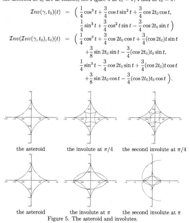
$J^{-1}$

Example 5.8 Let $\gamma$ : $[0,2\pi)arrow \mathbb{R}^{2}$ be the asteroid $\gamma(t)=(\cos^{3}t, \sin^{3}t)$ in

Example 4.9 and $t_{0}\in[0,2\pi)$. Then the involute and the second involute of

the asteroid at $t_{0}$ are as follows,

see

Figure 5 at $t_{0}=\pi/4$ and at _{$t_{0}=\pi.$}

$\mathcal{I}\prime nv(\gamma, t_{0})(t) = (\frac{1}{4}\cos^{3}t+\frac{3}{4}\cost\sin^{2}t+\frac{3}{4}\cos 2t_{0}\cos t,$

$\frac{1}{4}\sin^{3}t+\frac{3}{4}\cos^{2}t\sin t-\frac{3}{4}\cos 2t_{0}\sin t)$

$\mathcal{I}nv(\mathcal{I}nv(\gamma, t_{0}), t_{0})(t)$ $=$ $( \frac{1}{4}\cos^{3}t+\frac{3}{4}\cos 2t_{U}\cos t+\frac{3}{4}(\cos 2t_{0})t\sin t$

$+ \frac{3}{8}\sin 2t_{U}\sin t-\frac{3}{4}(\cos 2t_{0})t_{0}\sin t,$ $\frac{1}{4}\sin^{3}t-\frac{3}{4}\cos 2t_{0}\sin t+\frac{3}{4}(\cos 2t_{0})t\cos t$

$+ \frac{3}{8}\sin 2t_{0}\cos t-\frac{3}{4}(\cos 2t_{0})t_{0}\cos t)$.

the asteroid the involute at $\pi/4$ the second involute at $\pi/4$

the asteroid the involute at $\pi$ the second involute at $\pi$

6

Relationship between

evolutes and involutes

of fronts

In this section,

we

discuss

on

relationship between the evolutes and the

in-volutes of fronts. Let $(\gamma, v)$ : $Iarrow \mathbb{R}^{2}\cross S^{1}$ be

a

Legendre immersion with

the curvature of the Legendre immersion $(l, \beta)$

.

Assume that $(\gamma, v)$ dose not

have inflection points, namely, $\ell(t)\neq 0$ for all $t\in I$

.

We give

a

justification

ofProposition 2.4 with singular points.

Proposition 6.1 Let $t_{0}\in I.$

(1) $\mathcal{E}v(\mathcal{I}\prime r\iota v(\gamma, t_{0}))(t)=\gamma(t)$

.

(2) $\mathcal{I}nv(\mathcal{E}v(\gamma), t_{0})(t)=\gamma(t)-(\beta(t_{U})/\ell(t_{0}))\nu(t)$ .

For

a

given Legendre immersion $(\gamma, v)$ : $Iarrow \mathbb{R}^{2}\cross S^{1}$,

we

consider the

existence condition of a Legendre immersion $(\tilde{\gamma}, \tilde{v})$ : $Iarrow \mathbb{R}^{2}\cross S^{1}$ such that

$\mathcal{E}v(\tilde{\gamma})(t)=\gamma(t)$ or $\mathcal{I}nv(\tilde{\gamma}, t_{0})(t)=\gamma(t)$ for

some

$t_{0}$. By using Proposition

6.1, we have the following result.

Proposition 6.2 (1)

_If

$\tilde{\gamma}(t)=\mathcal{I}nv(\gamma, t_{0})(t)+\lambda\mu(t),$$\tilde{\nu}(t)=J^{-1}(v(t))$

for

any $t_{0}\in I$ and $\lambda\in \mathbb{R}$, then $\mathcal{E}v(\tilde{\gamma})(t)=\gamma(t)$.

(2)

_If

$\tilde{\gamma}(t)=\mathcal{E}v(\gamma)(t),$$\tilde{v}(t)=J(\nu(t))$ and $t_{0}$ is

a

singularpoint

of

$\gamma$, then

$\mathcal{I}nv(\overline{\gamma}, t_{0})(t)=\gamma(t)$.

By Theorems

4.8

and 5.7,

we

have the following sequence of the evolutes

and the involutes of the front.

. . . $\mathcal{I}nvarrow(\mathcal{I}nv^{2}(\gamma, t_{0})(t), J^{-2}(\nu)(t))arrow(\mathcal{I}nv(\gamma, t_{0})(t), J^{-1}(v)(t))arrow$

$(\gamma(t), v(t))arrow(\mathcal{E}v(\gamma)(t), J(\nu)(t))\mathcal{E}varrow \mathcal{E}v(\mathcal{E}v^{2}(\gamma)(t), J^{2}(v)(t))arrow \mathcal{E}v$ .

..

(5)

It follows that the corresponding sequence of the curvatures of the

Leg-endre immersions (5) is given by

. . .

$arrow(P(t), \beta_{-2}(t))arrow(P(t), \beta_{-1}(t))arrow$

$(\ell(t), \beta(t))arrow(\ell(t), \beta_{1}(t))arrow(\ell(t), \beta_{2}(t))arrow\cdots$ (6)

Moreover,

we

may suppose that $t$ is the arc-length parameter for $v$,

see

\S 3.

It follows that $l(t)=1$ for all $t\in I$, if necessary, a change of parameter

$t\mapsto-t$

.

Then the relationship between second components ofthe curvatures

of the Legendre immersions (6) is pictured

as

follows:

. . .

$arrow\int_{t_{0}}^{t}(\int_{t_{0}}^{t}\beta(t)dt)dtarrow\int_{t_{0}}^{t}\beta(t)dtarrow\beta(t)arrow\frac{d}{dt}\beta(t)arrow\frac{d^{2}}{dt^{2}}\beta(t)arrow\cdots$

Thisis corresponding to the relationship between the differential and integral

References

[1] V. I. Arnol’d, S. M. Gusein-Zade and A. N. Varchenko, Singulari ties

_of

Differentiable

Maps vol. I. Birkh\"auser (1986).

[2] V. I. Arnol’d, Singulari ties

_of

Caustics and Wave Fronts. Mathematics and

Its Applications 62 Kluwer Academic Publishers (1990).

[3] J. W. Bruce and P. J. Giblin, Curves and singularities. A geometri.cal

in-troduction to singularity theory. Second edition. Cambridge University Press,

Cambridge (1992).

[4] J. Ehlers and E.T. Newman, The theory

_of

caustics and wave

_front

singular-ities with physical applications, J. Math. Physics 41 (2000), 3344-3378.

[5] T. Fukunaga and M. Takahashi, Existence and uniqueness

_for

Legendre

curves. to appear in J. Geometry (2013).

[6] T. Fukunaga and M. Takahashi, Evolutes

_{of fronts}

in the Euclidean plane.

Preprint, Hokkaido University Preprint Series, No.1026 (2012).

[7] T. Fukunaga and M. Takahashi, Involutes

_{of fronts}

in the Euclidean plane.

Preprint, (2013).

[8] C. G. Gibson, Elementary geometry

_of

_{differentiable}

curves. An

undergradu-ate introduction. Cambridge University Press, Cambridge (2001).

[9] V. V. Goryunov and V. M. Zakalyukin, Lagrangian and Legendrian

singulari-ties, Real and complex singularities, Rends Math., Birkhauser, Basel, (2007),

169-185.

[10] A. Gray, E. Abbena and S. Salamon, Modem

_differential

geometry

_of

curves

and

_surfaces

with Mathematica. Third edition, _{Studies in Advanced}

Mathe-matics. Chapman and Hall/CRC, Boca Raton, FL (2006)

[11] E. Hairer and G. Wanner, Analysis by $it_{\mathcal{S}}$ history, Springer-Verlag, New

York,

(1996).

[12] W. Hasse, M. Kriele and V. Perlick, Caustics

_of

_wavefronts

in general rela-tivity, Class. Quantum Grav. 13 (1996), 1161-1182.

[13] C. Huygens, Horologium oscillatorium sive de motu pendulorum ad horologia

aptato _{demonstrationes} geometr$\dot{v}$cae, (1673).

[14] G.Ishikawa, Zariski‘smoduli problem forplane branches and the

_{classification}

of

Legendre curve singularities. Real and complex singularities, World Sci.

[15] S. Izumiya,

_Differential

Geometry

_from

the viewpoint

_of

Lagmngian or

Legen-dri an singularity theory. in Singularity Theory (ed., D. Ch\’eniot et al), World

Scientific (2007), 241-275.

[16] S. Izumiya and M. Takahashi, Spacelike pamllels and evolutes in Minkowski

pseudo-spheres. Journal of Geometry and Physics. 57 (2007), 1569-1600.

[17] S. Izumiya and M. Takahashi, Caustics and wave

_front

propagations:

Appli-cations to

_differential

geometry. Banach Center Publications. Geometry and

topology ofcaustics. 82 (2008), 125-142.

[18] S. Izumiya and M. Takahashi, On caustics

_{of submanifolds}

and canal

hyper-surfaces

in Euclidean space. Topology Appl. 159 (2012), 501-508.

[19] G. de l’Hospital, Analyse des

_Infiniment

Petits pour l’Intelligence des Lign es

Courbes, (1696).

[20] I. Porteous, Geometric

_{differentiation.}

For the intelligence

_of

curves and

surfaces.

Second edition. Cambridge University Press, Cambridge (2001) [21] M. Takahashi, Caustics and wave

_front

propagations. Singularity theory

of smooth maps and related geometry, Suurikenn Kokyuroku 1707 (2010),

135-148.

[22] G. Wassermann, Stability

_of

Caustics. Math. Ann. 216 (1975), 43-50.

[23] V. M. Zakalyukin, Reconstructions

of fronts

and caustics depending on a

pammeter and versality

of

mappings. J. Soviet Math. 27 (1983), 2713-2735.

[24] V. M. Zakalyukin, Envelope

_of

Families

_of

Wave Fronts and Control Theory.

Proc. Steklov Inst. Math. 209 (1995), 114-123.

Masatomo Takahashi,

Muroran Institute of Technology, Muroran 050-8585, Japan,