混合距離理論を用いた対流のモデル化 (乱流による輸送,拡散,混合の数理)

Modelling

for

Convective

Heat

Transport

Based

on

Mixing Length Theory

混合距離理論を用いた対流のモデル化

Yasuko

Yamagishi and

Takatoshi

Yanagisawa

山岸保子・柳沢孝寿

Institute for

Frontier

Research

on

Earth Evolution

固体地球統合フロンテイア研究システム

Japan

Marine

and

Science

Technology

Center

海洋科学技術センター

$lnloal\iota t\dot{w}n$

Convectionis the mostimportantmechanismfor the Earth’sinternaldynamics, andplays asubstantial role in

its evolution. Wheninvestigatingthe thermalhistoryof theEarth,convectiveheattransportshould be taken into account. However, it isdifficult to treatprecisely full

convective

flow throughout theEarth’s

entire

history. As

aresult, parameterized convection

was

developed and has beenwidelyused [Schubertet$\mathrm{a}/.$, 1979; Sharpeand

Peltier, 1979].

Convection occurringin the Earth’s

interior

has

some

complicatedaspects, including alargevariation in

vis-cosity,internal heating, and phaseboundaries. Inparticular,the viscosity contrast has asignificant effect

on

the

efficiencyofconvectiveheat transport. Parameterized

convection

treatsviscosity variation artificially, and

there-forehasmanylimitations. We developed

an

alternative method basedonthe conceptof“mixing length theory”.

The basic concept of this theory is thatheatis transported by verticalmotionofafluidparcel,and aftermigrating

for mixing length, the parcel loses it’s individuality. We

can

relate the local thermal gradient to the localconvective velocity of the fluidparcelanddefinetheeffective thermal

diffusivity

as

theeffectofconvective heat transport.

Then,

_{we can}

calculateahorizontaly averaged temperature profile and heat flux inaconvective fluid by solving

amere

thermal conductionproblem. Whenestimating the parcel’s velocity,

we

can

include effects such

as

that causedby variable viscosity.

In this study, through comparisonwith experimental results,

we

confirmthat the temperatureprofile

can

be calculated correctlybythismethod. Wefurther determine the effectoftheviscosity contrast

on

the temperature structure oftheconvectivefluid,and calculate the relationship between the Nusseltnumberandarepresentative

Rayleigh number for thelayer.

Fomuktion

As describedabove, here

we

simply treatthe

convective

heat flowusing mixing length theory, ofwhichthe

basicpremiseis that the velocity ofthefluid parcel is related to the local thermal gradient.

Mixing length theory

was

firstly developedin the field ofastrophysical studies in order toestimateheat flux

forconvective fluid with low Prandtl number andhigh Rayleighnumber [Vitense, 1953]. Thisformulation

was

derived by neglecting viscous drag, and the vertical velocity of the

convective

fluid parcel

was

estimated from free

fall velocitybyconsideringthatallgravitational

energy

was

changed intokinematic

energy.

The viscosity, then,

does not

appear

intheformula. Sasaki and

Nakazawa

[1986]and$Abe$[1993]extended thetheoryand formulated

forhighlyviscous fluids. Thisfomlulatim

was

based

on

theestimationof the verticalvelocity of aparcelfrom

Stokesvelocity, namely

on

theconceptthat the buoyancyforce is balancedwithviscousdrag. Theseformulations

were

derivdfrom theperturbation equationsof

energy

andmomentum

数理解析研究所講究録 1339 巻 2003 年 139-144

Inthis study,

we

$\mathrm{r}\mathrm{e}$-formulate this theory

more

simply and intuitively, especially for highly viscous flfluids.

Be-cause

the_{idea of this theory is that the flfluid parcel migrates for}amixing length_{and loses it’s individuality, the}

mixinglength

can

be regarded

as a

typeof

mean

free path. Therefore,the effectivethermal diffusivity, $\kappa_{c\circ nv\prime}$

can

bedeflflned

as

(2)

$\kappa_{\mathrm{c}onv}=v\mathrm{x}$$l$ (1)

where$v$is the velocity of theflfluidparcel, and$l$isthemixinglength. The temperaturedifference between theparcel

and thesurrounding$\mathrm{t}\mathrm{e}\mathrm{m}\mu \mathrm{r}\mathrm{a}\mathrm{t}\mathrm{u}\mathrm{r}\mathrm{e}$ oftheflfluid,generated becausethe parcel

moves

for

$l$vertically, is estimated

as

$\triangle T=[(\frac{dT}{dz})_{ad}-(\frac{dT}{dz})]l$

(4)

where $( \frac{dT}{dz})_{ad}$isthe adiabatic temperaturegradient.Inthisstudy, thesize of theparcelisassumed to$\mathrm{k}$identified

with the mixing length. $\Pi \mathrm{e}$ flfluidparcel

moves

against Stoke’s resistance. The velocity of the parcel, then, is

defind

as

$v$ $=$ $\frac{4\alpha gl^{2}}{15\nu}\triangle T$ (3)

$=$ $\frac{4\alpha g}{15\nu}[(\frac{dT}{dz})_{ad}-(\frac{dT}{dz})]l^{3}$

(5)

where$\alpha$isthethemalexpansivity,_$g$is the gravitationalaccerelation,and$\nu$is the$\mathrm{k}\mathrm{i}\mathrm{n}\mathrm{e}\mathrm{m}\mathrm{a}\dot{\mathrm{u}}\mathrm{c}$ viscosity. Theeffective

thermal diffisivityand_{convective heat flflux}

are

calculated

as

follows;

$\kappa_{conv}$ $=$ $v \mathrm{x}l=\frac{4\alpha g}{15\nu}[(\frac{dT}{dz})_{ad}-(\frac{dT}{dz})]l^{4}$

(6)

$J_{eonv}$ $=$ $\rho C_{P}\kappa_{conv}\frac{\triangle T}{l}=\rho C_{P}\kappa_{conv}[(\frac{dT}{dz})_{ad}-(\frac{dT}{dz})]$

where$\rho$isthe densityand$C_{P}$is the heatcapacity. Therefore, the temporal change of the horizontally averagd

$\mathrm{t}\mathrm{e}\mathrm{m}\mu \mathrm{r}\mathrm{a}\mathrm{t}\mathrm{u}\mathrm{l}\mathrm{e}$profileinthe

$\mathrm{c}\mathrm{o}\mathrm{n}\mathrm{v}\mathrm{e}\mathrm{c}\dot{0}\mathrm{v}\mathrm{e}$flfluid

can

beestimatedby solving theconduction equation,

$\rho C_{P}\frac{\partial T}{\partial t}=\mathrm{d}\mathrm{i}\mathrm{v}(k\frac{\partial T}{\partial z}-J_{conv})+H$ (7)

where$\mathrm{H}$is the

heatgeneration. Theseformulae

are

the

same

as

thosederivedbySasakiand

Nakazawa

[1986],

except forthecoefficient,althoughthe

process

of_formulationisdifference

convective

heatflux

In thismethd, the mixing length $\prime l’$ isthe most important parameter. We

assume

thatthemixinglengthis

qual to the distancefromthe boundary,

as

adoptedbySasakiand

Nakazawa

[1986]and$Abe$$[1993]$

.

$\mathrm{T}\mathrm{i}\mathrm{s}$

means

that the flfluid parcel has

a

sizethat is the

same as

the distance from the boundarytoits generating point, and it

moves

for the distanceof its size. This concept isillustratedinFigure 1. To

compare

with$\mathrm{e}\mathrm{x}\mu \mathrm{r}\mathrm{i}\mathrm{m}\mathrm{e}\mathrm{n}\mathrm{t}\mathrm{a}\mathrm{l}$ results,

we

setthe adiabatic temperature gradient to

zero

andcalculatedthe heatflflux based

on

equation (6). We assumed that the

viscosity

in the flfluid layer

was

constant._{Figure 2}shows theNusselt_numberderived by thecalculated heat

flflux

as a

function of Rayleighnumber. TheNusselt numberincreasesinproportiontotheRayleighnumber to the

$\mu \mathrm{w}\mathrm{e}\mathrm{r}$of$\frac{1}{3}$

:

$Nu$ $\propto$

$Ra^{\beta}$ (8)

$\beta$ $=$ $\frac{1}{3}$ (9)

$\mathrm{H}1:$ The concept of themixinglength andtheparcelsize,whentheparcel size is regarded

as

same

as

the mixing lengthandthemixing length is assumedto$\mathrm{k}$the distancefrom theboundaryofthe

convective

flluid.

10 $\mathrm{z}\ovalbox{\tt\small REJECT}-$ $10$

:

$\underline{\vee}$ 10 $\not\leqq$

101

1 1

$\mathrm{R}\bullet \mathrm{y}\mathrm{l}\mathrm{e}\mathrm{t}\iota \mathrm{h}\mathrm{N}\mathrm{n}\mathrm{m}\mathrm{b}\mathrm{e}\mathrm{r}$

$\mathrm{H}$ $2$

:

Nusselt number-Rayleigh numberrelationobtainedbythe mixing lengththeory.

and

agrees

well with the

experimentally

measured value. Therefore, themethd for treating

convective

heat flflow

&velopedhere

can

calculate the temperaturesructulein theconvectivelayer accurately and easily. However,the

Nusselt number is slightlyoverestimatedbythis calculationat lowRayleigh numbers. If the.Rayleigh number is

belowthecriticalRayleigh number, whichisthe value for the onset ofconvection,theNusselt numkr should$\mathrm{k}$

aunity. Here, thecalculatdNusseltnumber islarger than

1

underthecriticalRayleighnumber. This is because

in thismethM, the critical Rayleighnumberis 1, which is much smallerthan theexperimental

or

linear stable analytic $\mathrm{c}\mathrm{r}\mathrm{i}\dot{\mathrm{u}}\mathrm{c}\mathrm{a}\mathrm{l}$Rayleigh number $(\sim 10^{3})$

.

But the surplus heat flflux is relatively small and cannot affect the

system significantly.

$\hslash m\mu mture\ \mu n\ neeofv\dot{u}$

eosl.y

$\ln$consideringmantleconvection,$\mathrm{v}\dot{\iota}\mathrm{s}\mathrm{c}\mathrm{o}\mathrm{s}\mathrm{i}\mathrm{t}\mathrm{y}$ is strongly variable duetoitstemperaturedependence. In

previous

parameterized convection$\mathrm{m}\iota\lambda \mathrm{e}\mathrm{l}\mathrm{s}$

.

it is implicitly assumedthat the

Nusselt-Rayleigh

numkr relationship is not

affected byspatial$\mathrm{v}\mathrm{a}\dot{\mathrm{n}}\mathrm{a}\dot{\mathrm{u}}\mathrm{o}\mathrm{n}$inviscosity.Whenusing viscosity calculated fromthe

mean

$\mathrm{t}\mathrm{e}\mathrm{m}\mu \mathrm{r}\mathrm{a}\mathrm{t}\mathrm{u}\mathrm{r}\mathrm{e}$

$\mathrm{k}\mathrm{t}\mathrm{w}\infty \mathrm{n}$the

top and the bottom boundary, it is experimentally found that although the viscosity$\mathrm{d}\mathrm{e}\mu \mathrm{n}\mathrm{d}\mathrm{s}$

on

$\mathrm{t}\mathrm{e}\mathrm{m}\mu \mathrm{r}\mathrm{a}\mathrm{t}\mathrm{u}\iota \mathrm{e}$, the

Nusselt-Rayleighnumberrelationship

is

the

same

as

forconstant viscosity

convaetion

[Booker, 1976;Richteret

$al.$,

1983},

Some experimentaland computational studies indicate that when the viscosity has

an

eXtlet1rly high

$\mathrm{N}$

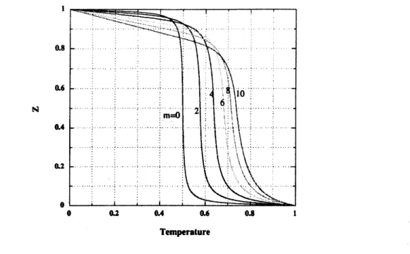
$\mathrm{T}\mathrm{e}\mathrm{m}\mu \mathrm{r}\cdot \mathrm{t}\mathrm{u}\mathrm{r}\mathrm{e}$

$\mathbb{H}$$3$

:

Horizontal

mean

temperatureprofileinconvective layerwithstronglytemperaturedependentviscosity. $\mathrm{m}$is

indicatorof temperature$\mathrm{d}\mathrm{e}\mu \mathrm{n}\mathrm{d}\mathrm{e}\mathrm{n}\mathrm{c}\mathrm{y}$ ofviscosity

contrast between the top and the bottomboundaries, the$\mathrm{d}\mathrm{e}\mu \mathrm{n}\mathrm{d}\mathrm{e}\mathrm{n}\mathrm{c}\mathrm{e}$ of Nusselt number

on

theRayleigh number

decreases [Christensen, 1984]. Namely, inequation(8),$\beta$drops klow $\frac{1}{3}$

.

In _{the method}

we

propose

here, only the local value of viscosity is _{needed. It is}

unnecessary

to calculate

theRayleigh number ofthe convective layer before gettingthe Nusselt number. Therefore, the variation of the

viscosity due to its temperature dependence

can

$\mathrm{k}$ taken into account directly, without

an

artificial treatment like parameterized

convection.

Inaddition,

as we

only solve

a

simpleconductionequation, lesscomputational

effort is needed,

even

though the $\mathrm{t}\mathrm{e}\mathrm{m}\mu \mathrm{r}\mathrm{a}\mathrm{t}\mathrm{u}\mathrm{r}\mathrm{e}$ dependence of viscosity

is

strong and

convection

is

very

active.

When the viscosity strongly depends

on

temperature, the2

or

3

dimensional calculations requireextremely large computational efforts, and therefore

are

difficult to

carry

out. Experiments

_are

also

more

difficult under such

situations. Consequently,the value of$\beta$hasnotkenclarified forconvectionwithhighly variable viscosity, and it

has not been determined whichviscosity is adequatefordefiningthe system’sRayleighnumber.

Figure3shows the temperatureprofiles in

a

convectivelayer with strongly temperature dependentviscosity. The

viscosityisgivenby

$\nu=\nu_{\mathrm{O}}\exp(-A(T-T_{\mathrm{O}}))$ (10)

where $T_{0}$ is the criterion $\mathrm{t}\mathrm{e}\mathrm{m}\mu \mathrm{r}\mathrm{a}\mathrm{t}\mathrm{u}\mathrm{r}\mathrm{e}$, which is usually assumed to be the temperature at the cold

or

the hot

boundary, and$\nu_{0}$is the viscosityat$T_{0}$

.

The indicator of the temperature dependence ofviscosity,$m$,isdefined by

$\frac{\nu(T_{t})}{\nu(T_{b})}=10^{m}$ (11)

where$T_{t}$ and$T_{b}$

are

the temperaturesatthetopand the bottomboundaries, $\mathrm{r}\mathrm{e}\mathrm{s}\mu \mathrm{c}\mathrm{t}\mathrm{i}\mathrm{v}\mathrm{e}\mathrm{l}\mathrm{y}$

.

Figure

3

indicates that

a

greater$m$ corresponds to

a

thicker surface conductive layer and

a

higher

core

temperature,

as

shown in 2-D

computationalcalculations[MoresiandSolomatov, 1995].

Next

we

used the methoddevelopdhere toestimate $\beta$ in equation(8), when the viscosity dependsstrongly

on

$\mathrm{t}\mathrm{e}\mathrm{m}\mu \mathrm{r}\mathrm{a}\mathrm{t}\mathrm{u}\mathrm{o}\mathrm{e}$

.

We

can

conffim that when the temperature $\mathrm{d}\mathrm{e}\mu \mathrm{n}\mathrm{d}\mathrm{e}\mathrm{n}\mathrm{c}\mathrm{e}$ of the viscosity baeomes strong, the

dependenceof the Nusselt numberon_{the Rayleigh number} decreases, namely $\beta$becomes smaller,

as

previou

$\mathrm{Z}^{\Xi}$

$\mathrm{R}\mathrm{a}$

$\overline{\cup\aleph}4$

:

Nusselt number-Rayleigh number relation with strongly temperature dependentviscosity. HereRayleigh

numberiscalculated by the

core

temperatureintheconvectivelayer

studiesindicated. Whenusingthe viscosityatthe bottom temperature to calculate the Rayleighnumber,the value of$\beta$decreases slightly from0.33to$\mathrm{a}\mathrm{r}\mathrm{o}\mathrm{u}\mathrm{n}\mathrm{d}0.3$

as

increasing_$m$

.

Bycontrast,inthe

case

of using theviscosityatthe

top boundary, thevalue of$\beta$gets muchsmaller below0.1. If the viscosity is estimatedatthe

core

temperature,$\beta$

changes from

0.330.24.

Figure 4showsthat relationship between the Nusselt number and theRayleighnumber,

for

a range

in thetemperaturedependence oftheviscosity,when theRayleigh number is estimated bytheviscosity at the

core

temperature.

lt isfound thatthevalue of$\beta$differs significantly between variousdefinitionsof the Rayleighnumber. If

we

wanttoinvestigatethe themal evolution of planetarybodies,the surface isthe only place where the viscosity

can

$\mathrm{k}$

put tobe constant throughout history. Thereforeit might be better to choose the_viscosity at thesurface of

the bodies to calculate the Rayleighnumber, Inthis

case.

the value of$\beta$to

use

would be much smaller than the

valueadopted by manyprevious studies. If the value of the

4

is assumedto be $\frac{1}{3}$ and the Rayleigh number is

estimatedfrom the viscosityatthe

mean

temperaturebetween the top and the bottomboundaries,theEarth would

havecooledveryrapidly. In the method developed in this study,

we

do not need

a

Rayleigh numbertocalculate the heat flux, andtherefore

we

arefree from thedefinition of

a

representative Rayleigh number and the value of

$\beta$

.

Appk.$M\dot{w}n$

for

the

themal history

of

the

$EMh$

In thisstudy,

we

developed

a

simple method fortreatingtheconvective heatflflux based

on

theconcept ofmixing

length theory, and showed that thismethod

can

calculate the temperature structureinthe

convective

layer conectly,

and

can

take intoaccount stronglytemperaturedependent viscosity

very

easily. Ofcourse, intemal heating

can

also be taken into account very easily by only adding

a

heatgeneration term to the $\mathrm{c}\mathrm{o}\mathrm{n}\mathrm{d}\mathrm{u}\mathrm{c}\dot{\mathrm{u}}\mathrm{o}\mathrm{n}$equation. As

described above,themixinglengthis the mostimportant parameterin thismethod, and byassumingthe mixing

length adequately, it is possible to extend this method to layeredconvection. In addition, it

can

be applied to

porous

media by

an

alterationtothe velocity of the fluid parcel. The mushy region ktween solidus and liquidus

can

be regarded

as a

$\mathrm{t}\mathrm{y}\mathrm{n}$of

porous

media, therefore, thisextended method

can

ueat the phase change regime in

theplanets. Thephase change also

can

be considered easily,throughthe simpleconductionproblem

we

solvein

this method. $\mathrm{T}\mathrm{e}\mathrm{m}\mu \mathrm{r}\mathrm{a}\mathrm{t}\mathrm{u}\mathrm{r}\mathrm{e}$

dependence

of the viscosity,

porous

media, phasechange, andlayered

convection: a1

of the obstaclestocalculating the thermal histories of the planetary bodies

can

be avoided by using this method.

Therefore,

we

argue

that thismethodis

an

adequate and powerful tool forinvestigatingthe

one

dimensional thermal

structural_{evolution of}the Earth.

$R_{6}ferences$

$\mathrm{A}\mathrm{k}$,Y.,Themal evolutionandchemical

differentiationofthe terrestrial

magma

ocean, in Evolution$cfth\ell$Eanh

andPlanets,E.Takahashi, R.Jeanloz, and D. Rubie,$\mathrm{e}\mathrm{d}\mathrm{s}.$,41-54,Geophysical Monograph.

$\mathrm{I}\mathrm{U}\mathrm{G}\mathrm{G}/\mathrm{A}\mathrm{G}\mathrm{U}$,

Washington D.C., 1$\mathfrak{B}3$

.

Booker, J.R.,?bemlalconvection with strongly temperature$\mathrm{d}\mathrm{e}\mu \mathrm{n}\mathrm{d}\mathrm{e}\mathrm{n}\mathrm{t}$ viscosity, J. FluidMech., 76, 741-754, 1976.

Christensen,U.R.,Heattransportby variable viscosity

convection

andimplications for the$\mathrm{e}\mathrm{a}[\mathrm{t}\mathrm{h}’\mathrm{s}$ thermal

evolu-tion, Phys. Earth Planet. Inter.,35,264-282,

_1986.

Moresi, L.-N., and V. S. Solomatov, Numerical investigation of$2\mathrm{D}$convection with extremely $1_{\mathfrak{B}}\mathrm{e}$ viscosity

variations,Phys. Fluids, 7, 2, 154-2, 162,

1995.

Richter,F.M.,H.-C.Nataf,andS.F.Daly, Heat transferand horizontallyaveraged_{temperature of}convection with

large viscosityvariations,J. FluidMech., $l2\mathit{9}$, 173-192,

1993.

Sasaki, S.,and K.Nakazawa, Metal-silicate fractionation inthegrowingearth:

energy

source

for the terrestrial

magma

ocean, J. Geophys. ${\rm Res}.,$$\mathit{9}l$,9,231-9,238,

1986.

Schubert,G.,P.Cassen,andR. E. Young, Subsolidusconvectivecmlinghistories of tenesaial planets, ICARUS,

$f\mathit{8}$, 192-211,

1979.

Sharpe,H.N.,and W.R.Peltier,_{A thermal history model}forthe Earth with pmmeteriaedconvoetion,Geophys. J. R.astr.

_Soc.f

59, 171-203, _1976.

Vitense, E.,Die

Wasserstoff

konvektionzone derSonne,$\mathrm{Z}$

Astrophys.,$f2$, 135-1U, _1993.