Validity of dimensional reduction in the random field O$(N)$ spin model for sufficiently large $N$(Applications of Renormalization Group Methods in Mathematical Sciences)

Validity

of

dimensional reduction in

the random

field

$\mathrm{O}(N)$

spin model

for

sufficiently large $N$

Yoshinori $\mathrm{S}\mathrm{a}\mathrm{k}\mathrm{a}\mathrm{m}\mathrm{o}\mathrm{t}\mathrm{o}^{1*},$Hisamitsu $\mathrm{M}\mathrm{u}\mathrm{k}\mathrm{a}\mathrm{i}\mathrm{d}\mathrm{a}^{2\uparrow}$,

and

Chigak Itoi3\ddagger

1 _Laborato

$\mathrm{r}y$

of

Physics, College

of

Science and Technology, Nihon University,

7-24-1

Narashino-dai, Funabashi-city, Chiba 274-8501, Japan

2 _Department

_of

_{Physics, Saitama Medical College, 981 Kawakado, Iruma-gun,}

Saitama 350-0496, Japan

3 _Department

_of

_{Physics, College}

_of

_{Science and Technology, Nihon University,}

1-8-14

Kanda-Surugadai, Chiyoda-ku, Tokyo 101-8308, Japan

Abstract

We study the critical phenomena of a random field $\mathrm{O}(N)$ spin model near the lower

criticaldimension, by means oftherenormalization group method and the $1/N$ expansion.

Wetreatthe$0(N)$ nonlinear$\sigma$model includinga randomfieldand all therandomanisotropy

terms, and calculate the one-loopbetafunctionfor a linear combinationofthem in$d=4+\epsilon$

under the assumption ofreplica symmetry. At first, we obtain all fixed points for the

one-loop beta function in the large $N$ limit, and discuss their stability. We find that thefixed

point yielding dimensional reduction is singlyunstable, and others arethefixed points with

many relevant modes,or unphysicalfixed point. Therefore,in the large$N$limit, the critical

phenomena in $4+\epsilon$ dimensions is found to be governed by the fixed point which gives

the result ofdimensional reduction. Next, we investigate the $1/N$ correction to the fixed

point yielding dimensional reduction. Careful analysis of the eigenvalue equation for the

infinitesimal deviationfrom thefixed pointisdoneat order $1/N$. In practice, thefixedpoint yielding dimensional reduction is found to be singly unstable. Thus, we conclude that the

dimensionalreduction holds forsufficientlylarge $N$

.

1

Introduction

Thecritical phenomena in the random field $\mathrm{O}(N)$ spin model is worth studying from the

view-point of quenched disorder and spin correlations. Dimensional reduction [1] isonekey to clarify

the nature of this model. Dimensional reduction claims that the critical behavior of the

d-dimensional random field $\mathrm{O}(N)$ spin modelis the

same

as of the $(d-2)$-dimensionalpure $\mathrm{O}(N)$

spin model, where $d$isthe spatial dimension. Dimensional reduction can predict the known

up-per critical dimension 6 for the random field $\mathrm{O}(N)$spin models $(N\geq 2)$, sincetheupper critical

dimension of the pure system are 4. It is thus natural to as$\mathrm{k}$ whetherthe dimensional

reduc-tion holds more precisely from six dimensions down to four. The strongversion ofdimensional

reduction claims that all critical exponents of the random field spin model in $d$ dimensions

are

identical to those of the corresponding pure model in $d-2$dimension. In some papers [2, 3, 4],

however, the breakdown of the dimensional reduction has been reported.

Since several rigorous results for the random field Ising model ($N=1$ case) indicated

the failureof the dimensional reduction to predict the lower critical dimensions [5, 6, 7], people

discussed the breakdown of dimensional reduction withsomeapproximation methods for random

field models. Fisher pointed out the breakdown of dimensional reduction due to the appearance

of the infinite number of relevant operators near four dimensions [2]. He showed the existence

of a fixed point yielding dimensional reduction for $N\geq 18$, but this fixed point is unstable

as

far asthe number of spin components$N$isfinite. Therefore, he concluded that thedimensional

$*\mathrm{y}\mathrm{o}\mathrm{s}\iota i$Ophys.$\mathrm{g}\mathrm{e}$

.

cat. nihon-u.$\mathrm{a}\mathrm{c}$

.

jp $\mathrm{t}_{-\mathrm{u}\mathrm{k}\mathrm{a}\mathrm{i}\mathrm{d}\mathrm{a}\mathrm{Q}\mathrm{s}\mathrm{a}\mathrm{i}\mathrm{t}\mathrm{a}\cdot \mathrm{a}}$

-med.$\mathrm{a}\mathrm{c}$

.

jp $\iota_{i\mathrm{t}\mathrm{o}\mathrm{i}\mathrm{O}\mathrm{p}\mathrm{h}\mathrm{y}\mathrm{s}.\mathrm{c}\mathrm{s}\mathrm{t}}$

.

nihon-u.$\mathrm{a}\mathrm{c}$

.

jp

reduction was not valid near four dimensions. M\’ezard and Young also suggested breakdown of dimensional reduction by replica symmetry breaking [3]. Now, many researchers believe that the dimensional reduction is incorrect in dimensions less than 6.

Recently, Tarjus and Tissier study the critical phenomena of this model in any dimension

and for any value of $N$ by using the nonperturbative renormalization group method and the

replicamethod [4]. Theyshow that there isacritical $N_{\mathrm{c}}$thedimensional reduction $\eta_{\mathrm{r}\mathrm{a}\mathrm{n}\mathrm{d}\mathrm{o}\mathrm{m}}(d)=$

$\eta_{\mathrm{p}\mathrm{u}\mathrm{r}\mathrm{e}}(d-2)$ is valid for $N\geq N_{c}$

.

Since they show $N_{\mathrm{c}}=18$ near the lower critical dimension,

their result does not

agree

with that ofthe references $[2, 3]$

.

To understandconsistency oftheir works, we reexaminetheone-loopbetafunction obtained

by Fisher employing the $1/N$-expansion method. Since Fisher did not solve the eigenvalue

problem for the stability around the fixed point, we solve this problem in a $1/N$ expansion.

First, in the large $N$ limit, we calculate all the fixed points including nonanalytic fixed points

as well as the fixed point yielding dimensional reduction. Then we investigate their stability

by solving the eigenvalue equation. We find that the only nontrivial stable fixed point yields

the dimensional reduction. Next, wecalculate the subleading correction to thefixed point, and

investigate the stability by solving the eigenvalue equation. We find that the unstable mode

pointed by Fisher is fictitious, and that the fixed point yielding the dimensional reduction is

practically singlyunstable in a coupling constant space of the given model with large $N$

.

This

result agrees with that by Tarjus and Tissier and a simple $1/N$-expansion. Thus, we conclude

that the dimensional reduction holds for sufficiently large $N$

.

In this note,

we

review these results obtained in our recent study [8].

This note is organized as follows. In Sec. 2, we briefly review the renormalization

group

analysis for the randomfield $0(N)$ spin modelin$4+\epsilon$dimensions, based onthereference[2]. In

Sec. 3, wecarefullyreexamine the critical phenomena of$(4+\epsilon)$-dimensional random field$\mathrm{O}(N)$

spin model in the large $N$ limit. As a result, in the large $N$ limit, the critical phenomenain

$4+\epsilon$ dimensions isshown to begoverned bythefixedpoint which givestheresultofdimensional

reduction. In Sec. 4, weinvestigate the $1/N$ correction to the fixed point yielding dimensional

reduction. We show that the fixed point yielding dimensional reduction is singly unstable.

Thus, weconclude that the dimensional reduction holds forsufficientlylarge $N$

.

Sec. 5 contains

conclusions.

2

Review

of

renormalization group

analysis

for

random fleld

$\mathrm{O}(N)$

spin model

in

$4+\epsilon$

dimensions

In this section, we briefly review the renormalization group analysisfor the random field $\mathrm{O}(N)$

spin model in $4+\epsilon$ dimensions, based on the reference [2]. We deal with the random field and

random anisotropy $\mathrm{O}(N)$ nonlinear $\sigma$ model which is known as an effective field theoretical

model for the random field $0(N)$ spin model near the lower critical dimension. We derive the

one-loop beta functions for the temperature and ageneral anisotropyincluding the randomfield

and random anisotropy terms, and obtain the fixed points of $\mathrm{O}(\epsilon)$

.

We calculate the critical

exponents $\eta$ and $\overline{\eta}$ for connected and disconnected correlation function. The stability of the

fixed points is discussed.

2.1

Model

We consider $\mathrm{O}(N)$ classical spins $S(x)$ with

a

fixed-length constraint $S(x)^{2}=1$

.

To take the

nonlinear $\sigma$ model of the following replica partition function and action:

$\mathcal{Z}=\int\prod_{\alpha=1}^{n}DS^{\alpha}\delta(S^{\alpha 2}-1)e^{-\beta H_{\mathrm{r}\mathrm{e}\mathrm{p}}}$,

$\beta H_{\mathrm{r}\mathrm{e}\mathrm{p}}=\frac{a^{2-d}}{2T}\int d^{d}x\sum_{\alpha=1}^{n}\sum_{\mu=1}^{d}(\partial_{\mu}S^{\alpha})^{2}-\frac{a^{-d}}{2T^{2}}\int d^{d}x\sum_{\alpha,\beta}^{n}R(S^{\alpha}\cdot S^{\beta})$, (2.1)

where $a$ is the ultraviolet cutoff, and the parameter $T$ denotes the dimensionless temperature.

The function $R(S^{\alpha}\cdot S^{\beta})$ represents general anisotropy including the random field and all the

random anisotropies, and is given by

$R(S^{\alpha} \cdot S^{\beta})=\sum_{\mu=1}^{\infty}\Delta_{\mu}(S^{\alpha}\cdot S^{\beta})^{\mu}$, (2.2)

where $\Delta_{\mu}$denotes the strength oftherandom field andthe$\mu$-th rank random anisotropy $(\mu=1$

is the random field, and $\mu\geq 2$ is the second and higher-rank random anisotropy).

2.2

Renormalization

group

We usethemethodobtained byPolyakov[9]for the pure system in $2+\epsilon$dimensions. Weexpress

each replica $S^{\alpha}(x)$ of the magnetization as a combination of fast fields $\varphi_{1}^{\alpha}$. $(x),$ $i=1,$

$\ldots,$$N-1$

and aslowfield $n_{0}^{\alpha}(x)$ of the unit length. We use the representation

$S^{\alpha}=n_{0}^{\alpha}\sqrt{1-\varphi^{\alpha 2}}+\varphi^{\alpha}$, $\varphi^{\alpha}=\sum_{:=1}^{N-1}\varphi_{\iota}^{\alpha}\epsilon_{i}^{\alpha}$, (2.3)

where the unit vectors $e_{\dot{\mathrm{t}}}^{\alpha}(x)$ are perpendicular to each other and also to the vector $n_{0}^{\alpha}(x)$

.

Substituting the equation (2.3) into the Hamiltonian (2.1) and selecting quadratic terms in

$\varphi^{\alpha}(x)$

,

we have

$\beta H_{\mathrm{r}\mathrm{e}\mathrm{p}}=\beta H_{\mathrm{u}\mathrm{n}\mathrm{p}\mathrm{e}\mathrm{r}\mathrm{t}}$

.

$+\beta H_{\mathrm{i}\mathrm{n}\mathrm{t}}+\beta H_{0}$, (2.4)

$\beta H_{\mathrm{u}\mathrm{n}\mathrm{p}\mathrm{e}\mathrm{r}\mathrm{t}}$. $= \frac{a^{2-d}}{2T}\int d^{d}x\sum_{\alpha=1}^{n}\sum_{\mu=1}^{d}(\partial_{\mu}n_{0}^{\alpha})^{2}-\frac{a^{-d}}{2T^{2}}\int d^{d}x\sum_{\alpha,\beta}^{n}R(n_{0}^{\alpha}\cdot n_{0}^{\beta})$ , (2.5) $\beta H_{\mathrm{i}\mathrm{n}\mathrm{t}}=\frac{a^{2-d}}{2T}\int d^{d}x\sum_{\alpha=1}^{n}\sum_{\mu=1}^{d}\{(\partial_{\mu}n_{0}^{\alpha})^{2}\cdot(-\sum_{i=1}^{N-1}\varphi_{i}^{\alpha 2})+\sum_{i,j}^{N-1}c_{\mu^{1}}^{\alpha}c_{\mu j}^{\alpha}\varphi_{1}^{\alpha}$

.

$\varphi_{j}^{\alpha}\}$

$- \frac{a^{-d}}{2T^{2}}\int d^{d}x\sum_{\alpha,\beta}^{n}\{A^{\alpha\beta}\sum_{i=1}^{N-1}\varphi_{i}^{\alpha 2}+\sum_{i,j}^{N-1}B_{ij}^{\alpha\beta}\varphi_{i}^{\alpha}\varphi_{j}^{\alpha}+\sum_{1,j}^{N-1}C_{ij}^{\alpha\beta}\varphi_{1}^{\alpha}$.$\varphi_{j}^{\beta}\}$

,

(2.6)

$\beta H_{0}=\frac{a^{2-d}}{2T}\int d^{d}x\sum_{\alpha=1}^{n}\sum_{\mu=1}^{d}\sum_{i=1}^{N-1}(\partial_{\mu}\varphi_{1}^{\alpha}$. $- \sum_{j=1}^{N-1}f_{\mu ij}^{\alpha}\varphi_{j}^{\alpha})^{2}$

,

(2.7)

where

$c_{\mu 1}^{\alpha}=(\partial_{\mu}n_{\mathrm{O}}^{\alpha})\cdot e_{i}^{\alpha}$

,

(2.8)

$A^{\alpha\beta}=-(n_{0}^{\alpha}\cdot n_{0}^{\beta})R’(n_{0}^{\alpha}\cdot n_{0}^{\beta})$, (2.9)

$B_{jj}^{\alpha\beta}=(n_{0}^{\beta}\cdot e_{\dot{2}}^{\alpha})(n_{0}^{\beta}\cdot e_{j}^{\alpha})R’’(n_{0}^{\alpha}\cdot n_{0}^{\beta})$

,

(2.10)

$C_{1j}^{\alpha\beta}.=(e^{\alpha}. .e_{j}^{\beta})|R’(n_{0}^{\alpha}\cdot n_{0}^{\beta})+(n_{0}^{\beta}\cdot \mathrm{e}_{i}^{\alpha})(n_{0}^{\alpha}\cdot e_{j}^{\beta})R’’(n_{0}^{\alpha}\cdot n_{0}^{\beta})$ , (2.11)

Here we put $f_{\mu ij}^{\alpha}(x)=0$

.

We turn to the perturbative renormalization

group

transformation. Representing the new

replicated Hamiltonian by $\beta H_{\mathrm{r}\mathrm{e}\mathrm{p}}’$, we have thefollowing expression for $\beta H_{\mathrm{r}\mathrm{e}\mathrm{p}}’$ up to the second

orderofthe perturbation expansion:

$\beta H_{\mathrm{r}\mathrm{e}\mathrm{p}}’\simeq\beta H_{\mathrm{u}\mathrm{n}\mathrm{p}\mathrm{e}\mathrm{r}\mathrm{t}}$

.

$+ \langle\beta H_{\mathrm{i}\mathrm{n}\mathrm{t}}\rangle_{0}-\frac{1}{2!}\langle\beta H_{\mathrm{i}\mathrm{n}\mathrm{t};}\beta H_{\mathrm{i}\mathrm{n}\mathrm{t}}\rangle_{0}$, (2.13)

where $\langle A;B\rangle_{0}=\langle AB\rangle_{0}-\langle A\rangle_{0}\langle B\rangle_{0}$, and $\langle\cdots\rangle_{0}$denotes the

average

defined by

$\langle\cdots\rangle_{0}=\frac{\int\prod_{\alpha=1}^{n}D\varphi^{\alpha}(\cdots)e^{-\beta H\mathrm{o}}}{\int\prod_{\alpha=1}^{n}D\varphi^{\alpha}e^{-\beta H_{0}}}$

.

(2.14)

Tocalculate the renormdization groupbeta function, we use a free propagator of the fluctuation

field

$\langle\varphi^{\alpha};(x)\varphi_{j}^{\beta}(y)\rangle_{0}=Ta^{d-2}G_{0}(x-y)\delta_{\alpha\beta}\delta_{jj}$ , (2.15)

$G_{0}(x-y)= \int\frac{d^{d}p}{(2\pi)^{d}}\frac{e^{ip\cdot(x-y)}}{p^{2}}$, (2.16)

$G_{0}(0)= \int\frac{d^{d}p}{(2\pi)^{d}}\frac{1}{p^{2}}$

$= \frac{S_{d}}{(2\pi)^{d}}\int_{b^{-1}}^{a^{-1}}dpp^{d-3}=\frac{S_{d}}{(2\pi)^{d}}\frac{a^{d-2}}{d-2}\{1-(\frac{b}{a})^{2-d}\}$

,

(2.17)

where $b$ is the ultraviolet cutoff; $b>a$

,

and $S_{d}=2\pi^{\frac{d}{2}}/\Gamma(d/2)$

.

At one-loop level, we have the

expressions for $\langle\beta H_{\mathrm{i}\mathrm{n}\mathrm{t}}\rangle_{0}$ and $\langle\beta H_{\mathrm{i}\mathrm{n}\mathrm{t};}\beta H_{\mathrm{i}\mathrm{n}\mathrm{t}}\rangle_{0}$:

$\langle\beta H_{\mathrm{i}\mathrm{n}\mathrm{t}}\rangle_{0}\simeq\frac{a^{2-d}}{2T}\{-(N-2)(Ta^{d-2})G_{0}(0)\}\int d^{d}x\sum_{\alpha=1}^{n}\sum_{\mu=1}^{d}(\partial_{\mu}n_{0}^{\alpha})^{2}$

$- \frac{a^{-d}}{2T^{2}}(Ta^{d-2})G_{0}(0)\int d^{d}x\sum_{\alpha,\beta}^{n}\{-(N-1)zR’(z)+(1-z^{2})R’’(z)\}$,

(2.18)

$- \frac{1}{2!}\langle\beta H_{\mathrm{i}\mathrm{n}\mathrm{t};}\beta H_{\mathrm{i}\mathrm{n}\mathrm{t}}\rangle_{0}\simeq\frac{a^{2-d}}{2T}(a^{d-4}\int dyG_{0}(y)^{2})\int d^{d}x\sum_{\alpha=1}^{n}\sum_{\mu=1}^{d}\{-(N-2)R’(1)(\partial_{\mu}n_{0}^{\alpha})^{2}\}$

$- \frac{a^{-d}}{2T^{2}}(\frac{a^{d-4}}{2}\int dyG_{0}(y)^{2})\int d^{d}x\sum_{\alpha,\beta}^{n}\{(N-2+z^{2})[R’(z)]^{2}$

$-2z(1-z^{2})R’(z)R’’(z)+(1-z^{2})^{2}[R’’(z)]^{2}-2(N-1)zR’(1)H(z)$

$+2(1-z^{2})R’(1)R’’(z)\}$

.

(2.19)

where

we

put $z=n_{0}^{\alpha}\cdot n_{0}^{\beta}$ for simplicity. If

we

define the

new

coupling constants by

$\beta H_{\mathrm{r}\mathrm{e}\mathrm{p}}’=\frac{b^{2-d}}{2T},$

$\int d^{d}x\sum_{\alpha=1}^{n}\sum_{\mu=1}^{d}(\partial_{\mu}n_{0}^{\alpha})^{2}-\frac{b^{-d}}{2T^{2}},\int d^{d}x\sum_{\alpha,\beta}^{n}\tilde{R}(z)$, (2.20)

we have theone-loop beta functions

$\frac{dR(z)}{dt}\equiv\partial_{t}R(z)$

$=(4-d)R(z)+AT\{2(N-2)R(z)-(N-1)zR’(z)+(1-z^{2})R’’(z)\}$

$+A(2(N-2)R’(1)R(z)-(N-1)zR’(1)R’(z)+(1-z^{2})R’(1)R^{N}(z)$

$+ \frac{1}{2}[R’(z)]^{2}(N-2+z^{2})-R’(z)R’’(z)z(1-z^{2})+\frac{1}{2}[R’’(z)]^{2}(1-z^{2})^{2})$ , (2.22)

where $t=\ln(b/a)$, and $A=S_{d}/(2\pi)^{d}$

.

2.3

Critical

phenomena

in

$4+\epsilon$

dimensions

In $4+\epsilon$ dimensions, the one-loop beta functions $\partial_{t}T$ and $\partial_{t}R(z)$ become

$\partial_{t}T=-(2+\epsilon)T+A(N-2)T^{2}+A(N-2)TR’(1)$, (2.23)

$\partial_{t}R(z)=-\epsilon R(z)+AT\{2(N-2)R(z)-(N-1)zR’(z)+(1-z^{2})R’’(z)\}$

$+A(2(N-2)R’(1)R(z)-(N-1)zR’(1)R’(z)+(1-z^{2})R’(1)R^{n}(z)$

$+ \frac{1}{2}[R’(z)]^{2}(N-2+z^{2})-R’(z)R’’(z)z(1-z^{2})+\frac{1}{2}[R’’(z)]^{2}(1-z^{2})^{2)}$

.

$(2.24)$

Solving the fixed-point equation $\partial_{t}T=0$, we find that there is no nontrivial fixed point for $T$

of$\mathrm{O}(\epsilon)$. Thus, we have only trivial fixed point $T=0$. Linearizing $\partial_{t}T$ around $T=0$, we have

$\frac{\partial(\partial_{t}T)}{\partial T}|_{T=0}=-2-\epsilon+A(N-2)R’(1)$

.

(2.25)

Since $R’(1)$ is at most of order $\epsilon,$ $\partial(\partial_{t}T)/\partial T|\tau=0$ is negative. Thus, the renormalization group

flows around a zerotemperature go into the fixed point$T=0$

.

_{We put} $T=0$ below. Then the

one-loop betafunction $\partial_{t}R(z)$ becomes as follows:

$\partial_{t}R(z)=-\epsilon R(z)+A(2(N-2)R’(1)R(z)-(N-1)zR’(1)R’(z)+(1-z^{2})R’(1)R’’(z)$

$+ \frac{1}{2}[R’(z)]^{2}(N-2+z^{2})-R’(z)R’’(z)z(1-z^{2})+\frac{1}{2}[R’’(z)]^{2}(1-z^{2})^{2})$

.

(2.26)

Expanding $R(z)$ about the aligned state with $z=1$ for all a, $\beta$, we obtain the one-loop beta

functions for $R’(1),$ $R”(1)$ at zero-temperature fixed point:

$\partial_{t}R’(1)=-\epsilon R’(1)+A(N-2)R^{l}(1)^{2}$, (2.27)

$\partial_{t}H’(1)=-\epsilon R’’(1)+A[6R’(1)R’’(1)+(N+7)R’’(1)^{2}+R’(1)^{2}]$

.

(2.28)

The beta functions (2.27) and (2.28) have two nontrivial fixed points:

$(R’(1), R_{+}’’(1))$ $=$ $( \frac{\epsilon}{A(N-2)},$ $\frac{(N-8)+\sqrt{(N-2)(N-18)}}{2A(N-2)(N+7)}\epsilon)$

,

(2.29)

$(R’(1), R_{-}’’(1))$ $=$ $( \frac{\epsilon}{A(N-2)},$ $\frac{(N-8)-\sqrt{(N-2)(N-18)}}{2A(N-2)(N+7)}\epsilon)$

.

(2.30) The formulasfor the critical exponents$\eta$ and $\overline{\eta}$

enable us to obtain

$\overline{\eta}=\eta=\frac{\epsilon}{N-2}$

.

(2.32)

This result of$\eta$ is consistent with that of a pure system in $d=2+\epsilon$ up toorder

$\epsilon$

.

The result

$\overline{\eta}=\eta$confirms the dimensional reduction. From the fixed point (2.29) and (2.30), we find that

these results are applicable only for $N\geq 18$

.

Feldman carefully reexamined the one-loop beta

function, and found nonanalytic fixed points which control the critical phenomena instead of

the fixed point (2.29) and (2.30) [10]. He calculated the exponents $\eta$ and $\overline{\eta}$ for $N=3,4,5$ in

$4+\epsilon$ dimensions numerically:

$\eta=5.5\epsilon$

,

$\overline{\eta}=10.1\epsilon$, for $N=3$

$\eta=0.79\epsilon$

,

$\overline{\eta}=1.4\epsilon$, for $N=4$ (2.33)

$\eta=0.42\epsilon$, $\overline{\eta}=0.70\epsilon$

,

for $N=5$

Then he concluded that dimensional reduction breaks down near four dimensions for several

finite $N$

.

Theeigenvalues of the scaling matrix at the fixed points (2.29) and (2.30) are

$\lambda_{1}$ $=$ $+\epsilon$, (2.34)

$\lambda_{2}^{\pm}$ _$=$ $\pm\epsilon\sqrt{\frac{N-18}{N-2}}$

.

(2.35)

Thus, the fixed point (2.29) is unstable. The fixed point (2.30) seems to be stablefor $N\geq 18$

.

However, Fisher showed that the fixed point (2.30) is also unstable [2]. His statement is as

follows. Expanding $R(z)$ about the aligned state with $z=1$ up to the k-th order, we have the

one-loop beta function for $R^{(k)}(1)$

.

Substitutingthefixed point $(R’(1)^{*}, R_{-}’’(1)^{*},$

$\ldots,$$R^{(k-1)}(1)^{*})$

into the beta function for $R^{(k\rangle}(1)$

,

we

can

obtain the nontrivial fixed point $R^{(k)}(1)^{*}$ at $0(\epsilon)$

.

The eigenvalue at the fixed point is given by

$\lambda_{k}=\epsilon(\frac{2k^{2}-k(N-1)+2N-4}{N-2}-1)$

$\simeq\epsilon((1-k)\epsilon+\frac{2k^{2}-k}{N})$ , (2.36)

for $k\geq 3$

.

The eigenvalue is found to be positive for large $k$

.

Then Fisher concluded that

there is no singly unstable fixed point, and the dimensional reduction breaks down near four

dimensions. In Sec. 4, we show thatthe infinitely many relevant modes pointed out by Fisher

are unphysical modes.

In the next section, we carefully reexamine the critical phenomena of $(4+\epsilon)$-dimensional

randomfield $\mathrm{O}(N)$ spin model in the large $N$ limit.

3

Large

$N$

limit

We take the large $N$ limit with _$NR(z)$ finite, and redefine $R(z)$ as follows: $NR(z)arrow R(z)$

.

Thus, theone-loop beta function for $R(z)$ becomes

3.1

Fixed

points

Following the method given by Balents and Fisher [11], we consider the flowequation for $R’(z)$

instead ofthat for $R(z)$

.

Differentiating theone-loop beta function with respect to $z$, we have

$\partial_{t}R’(z)=-\epsilon R’(z)+A(R’(1)R’(z)-zR’(1)R’’(z)+R’(z)R’’(z))$

.

(3.2)

We redefine the parameters

as

follows:

$R’(z) \equiv\frac{\epsilon}{A}u(z)$, $t’\equiv\epsilon t$, _{$u(1)\equiv a$}

.

(3.3)

The one-loop beta function becomes

$\partial_{t’}u(z)=(a-1)u(z)-zau’(z)+u(z)u’(z)$

.

(3.4)

Here, we consider the fixed-point equation

$0=(a-1)u(z)-zau’(z)+u(z)u’(z)$

.

(3.5)

Substituting $z=1$ into the equation (3.5), we have two fixed points

$a=0,1$

.

(3.6)

Solving the differential equation (3.5) under the condition $a=1$, we have two nontrivial

solutions:

$u(z)=1,$$z$

.

(3.7)

In the case of$u(z)=1$,

we

have

$R(z)= \frac{\epsilon}{A}(z-\frac{1}{2})$

.

(3.8)

It indicates that

$( \Delta_{1}, \Delta_{2})=(\frac{\epsilon}{A},$ $0)$, (3.9)

$(R’(1), R”(1))=( \frac{\epsilon}{A},$$0)$

.

(3.10)

Thus, the solution (3.8) is the “random field solution”. In the caseof $u(z)=1$, we have

$R(z)= \frac{\epsilon}{2A}z^{2}$

.

(3.11)

It indicates that

$(\Delta_{1}, \Delta_{2})=(0,$$\frac{\epsilon}{2A})$, (3.12)

$(R’(1), R”(1))=( \frac{\epsilon}{A’}\frac{\epsilon}{A})$

.

(3.13)

Thus,thesolution (3.11)is notthe “random field$\mathrm{s}\mathrm{o}\mathrm{l}\mathrm{u}\mathrm{t}\mathrm{i}\mathrm{o}\mathrm{n}" \mathrm{b}\mathrm{u}\mathrm{t}$the “randomanisotropy solution”.

Ifwe solve the differential equation (3.5) under the condition $a=0$, the nontrivial solution

isobtained

as

follows:

From the solution (3.14), we have

$R(z)= \frac{\epsilon}{2A}(z-1)^{2}$

.

(3.15)

It indicates that

$( \Delta_{1}, \Delta_{2})=(-\frac{\epsilon}{A},$ $\frac{\epsilon}{2A})$

,

(3.16)

$(R’(1), R”(1))=(0,$$\frac{\epsilon}{A})$

.

(3.17)

Thus, the solution (3.15) is unphysical.

We turn to the general $a$. If$a\neq 0,1$

,

$\frac{du(z)}{dz}=\frac{(a-1)u(z)}{za-u(z)}$

.

(3.18)

Taking theinversion, we regard $z$ as a function of$u$

.

One gets

$\frac{dz(u)}{du}=\frac{az(u)}{a-1u}-\frac{1}{a-1}$, (3.19) which is easily integrated. The result is

$z(u)=C|u|^{\frac{a}{a-1}}+u$

.

(3.20)

The constant $C$ is fixed by putting $z=1$ as follows:

$C=(1-a)|a|^{-\frac{\mathrm{o}}{a-1}}$

.

(3.21)

Then, we have

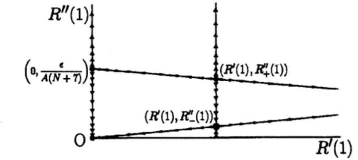
$z=u-(a-1)| \frac{u}{a}|^{\frac{a}{a-1}}$ (3.22)

Now we revert (3.22) to the solution $u(z)$ for (3.18). Because $z(u)$ takes the maximum value 1

at $u=a,$ $u(z)$ is double valued as we show in Fig. 3.1. It is seen from (3.18) that $du/dz$ is ill

defined on $u=az$

.

Therefore the lower branch terminates at the origin, so that it should be

continued to the region $-1\leq z<0$

.

This is possible only if$a/(a-1)$ is a positive integer.

Figure 3.1: A schematic graph of$u(z)$

.

Since the derivative of$u$ is ill defined

on

$u=az$, the

Expanding $u$ around $a$

,

we have

$z=u-(a-1)| \frac{u}{a}|^{\frac{a}{a-1}}$

$=a+(u-a)-(a-1)(1+ \frac{u-a}{a})^{\overline{a}\overline{1}}\underline{\mathrm{B}}$

$\simeq 1-\frac{1}{2a(a-1)}(u-a)^{2}$

.

(3.23)

Since-l $\leq z\leq 1$

,

we have

$1-z \simeq\frac{(u-a)^{2}}{2a(a-1)}\geq 0$

.

(3.24)

Thus, we find that the fixed point $a$ must be $a\geq 1$

.

In practice, in the case of$0\leq a<1$, the

critical exponent $\overline{\eta}$ becomes negative. In the case of $a>1$, the equation (3.24) is rewritten as

follows:

$u(z)\simeq a\pm\sqrt{2a(a-1)(1-z)}$

.

(3.25)

Note that the plus (minus) sign in front of the square root means to take the upper (lower)

branch. Differentiating the above equation by$z$

,

we have

$u’(z)\simeq\mp\sqrt{\frac{a(a-1)}{2}}(1-z)^{-1/2}$

.

(3.26)

We find that $u’(z)$ diverges as $zarrow 1$

.

Thus,the fixed point$a>1$ is called the nonanalyticfixed

point. In contrasttoit, the fixed points (3.8) and (3.11) are called the analytic fixed points.

3.2

Stabilities

of

the fixed-point

solutions

Next,

we

study the stability ofthe fixed points. Let $u(z)^{*}$ be a fixed point solution:

$0=u(z)^{*}(a^{*}-1)+u’(z)^{*}(u(z)^{*}-a^{*}z)$

.

(3.27)

We put $u(z)^{*}arrow u(z)^{*}+v(z)$ and $a^{*}arrow a^{*}+b$, and studythe behavior of thefirst order in $v(z)$

and $b$:

$v(z)(a-1)+u(z)b+v’(z)(u(z)-az)+u’(z)(v(z)-bz)=\lambda v(z)$

.

(3.28)

Here,

we

omit the$\mathrm{a}\mathrm{s}\mathrm{t}\mathrm{e}\mathrm{r}\mathrm{i}\mathrm{s}\mathrm{k}*\mathrm{f}\mathrm{o}\mathrm{r}$brevity. $\lambda$denotes theeigenvalue. The negativeeigenvalue$\lambda<0$

indicates that the fixed-point solution is stable, and the positive eigenvalue $\lambda>0$indicates that

the fixed-point solution is unstable. Normalizing $v(z)$ appropriately, we can take $v(1)=0$ or

$v(1)=1$

.

3.2.1 $R(z)=\epsilon(z-1/2)/A$

For $a=1$ and $u(z)=1$, the equation (3.28) becomes

$b+v’(z)(1-z)=\lambda v(z)$

,

(3.29)

where $b$represents _$v(1)$ taking$0$ or 1. When $b=0$

,

the solution is

where $\lambda<0$ because of the initial condition $b=v(1)=0$

.

On the other hand, when $b=1$, a

general solution is

$v(z)=\{$ $\lambda^{-1}+c(1-z)^{-\lambda}$ $(\lambda\neq 0)$,

$\ln|1-z|$ $(\lambda=0)$

.

(3.31)

Here the condition $b=1$ requires that $\lambda=1$ and $c=0$

.

In conclusion, theallowed value of$\lambda$ is

$\lambda<0$or $\lambda=1$

.

This shows that the fixed-point solutionis singly unstable.

3.2.2 $R(z)=\epsilon z^{2}/(2A)$

For $a=1$ and $u(z)=z$, the equation (3.28) becomes

$v(z)=\lambda v(z)$

.

(3.32)

Then, $\lambda=1$, and the fixed point is fully unstable.

3.2.3 $R(z)=0$

Since $a=0$ and $u=0$ in thiscase, the equation (3.28) $\mathrm{i}\mathrm{s}-v(z)=\lambda v(z)$, which

means

$\lambda=-1$

for any $v(z)$; thus the trivial fixed point is fullystable.

3.2.4 Nonanalytic case

Next we turn to the nonanalytic case. Using the identity

$v’(z)= \frac{dv(u)}{du}\frac{du}{dz}$, (3.33)

the equation (3.28) is rewritten as follows:

$\frac{dv}{du}+f(u)v=g(u)$, (3.34)

$f(u)=-( \frac{1}{u}+\frac{1}{az-u}-\frac{\lambda}{(a-1)u})$, (3.35)

$g(u)=( \frac{1}{a-1}-\frac{z}{az-u})b$

.

(3.36)

Inthe case of $b=0$

,

_{the equation (3.34) becomes}

$\frac{dv}{du}+f(u)v=0$

.

(3.37)

Solving the above differential equation, we have

$v(u)=C \exp(-\int f(u)du)$

$=C \frac{|u(z)|^{\frac{-\lambda\neq a}{a-1}}}{|a^{\frac{1}{a-1}}-u(z)^{\frac{1}{a-1}1}}$

.

(3.38)

Accordingto the condition $v(u(1))=b=0$, the constant$C$ is fixed as $C=0;v(z)=0$

.

Hence,

thereare

no

nontrivial solutions satisfying $b=0$

.

Next, we consider the case of $b=1$

.

The solution of the differential equation (3.34) is

generally written as follows:

Then, we concentrate on the calculation of the integration in the curly bracket. The integrand

becomes

$g(u) \exp(\int f(u)du)=\pm\frac{u^{\frac{\lambda}{a-1}1}}{a(a-1)}$

.

(3.40)

Note that the plus sign is taken for the upper branch and the minus for the lower branch.

Insertingthis into (3.39), we get

$v(u)=\{$

$- \frac{\hat{u}^{a/(a-1)}}{\lambda}\frac{1-\hat{u}^{-\lambda/\langle a-1)}}{1-\hat{u}^{1/(a-1)}}$

$(\lambda\neq 0)$,

$\frac{\hat{u}^{a/(a-1)_{\ln\hat{u}}}}{(1-a)(1-\hat{u}^{\mathrm{l}/(a-1)})}$ $(\lambda=0)$,

(3.41)

where $\text{\^{u}}\equiv u/a$

.

Here the constant terms are chosen to satisfy $v(u(z))arrow 1$ as $zarrow 1$

.

Thus, the

deviation $v(u)$ from the upper branch is finite for any $\lambda$, because $\text{\^{u}}\geq 1$

.

On the contrary, $v(u)$

from the lower branch may diverge at $u=0$ and $-1$

.

We need a constraint on $\lambda$ for $v(u)$ to be

finite. We find that the lower branch with $a=3/2$ can be extended to $-1\leq z\leq 0$

,

and that

$v(u)$ remains finite for $\lambda=1$ or negative integers; namely, the lower branch with $a=3/2$ is

singly unstable. However, this fixed-point solution is unphysical because it does not satisfy the

Schwartz-Sofferinequality $2\eta\geq\overline{\eta}[12]$

.

This inequality requires$a=1+\mathrm{O}(1/N)$

.

Other physical

lower-branch fixed points satisfying the Schwartz-Soffer inequality has many relevant modes of

$\mathrm{O}(N)$

.

4

Subleading

corrections

4.1

The

fixed point

Here,

we

calculate the subleading correction to the analytic fixed point $R(z)=(\epsilon/A)(z-1/2)$

and the eigenfunctions. We expand the fixed-point solution

$R(z)= \frac{1}{N}R_{0}(z)+\frac{1}{\mathit{1}\mathrm{V}^{2}}R_{1}(z)+\mathrm{O}(\frac{1}{N^{3}})$

,

(4.1)

and calculatethe subleading correction $R_{1}(z)$

.

Substituting this expansion into (2.26), weobtain

$\partial_{t}R_{1}(z)=-\epsilon R_{1}(z)+A(2R_{1}’(1)R_{0}(z)+2R_{0}’(1)R_{1}(z)-zR_{1}’(1)R_{0}’(z)-zR_{0}’(1)R_{1}’(z)$ $+R_{1}’(z)R_{0}’(z)-4R_{0}’(1)R_{0}(z)+zR_{0}’(1)R_{0}’(z)+(1-z^{2})R_{0}’(1)R_{0}’’(z)$

$+ \frac{1}{2}(z^{2}-2)R_{0}’(z)^{2}-R_{0}’(z)R_{0}’’(z)z(1-z^{2})+\frac{1}{2}R_{0}’’(z)^{2}(1-z^{2})^{2)}$

.

We substitute the unique singly unstable fixed-point solution

$R_{0}(z)= \frac{\epsilon}{A}(z-\frac{1}{2})$

intothe above equation; then weobtain afixed-point equation for the correspondingcorrection

$R_{1}(z)$,

$(1-z)R_{1}’(z)+R_{1}(z)-(1-z)R_{1}’(1)+ \frac{\epsilon}{A}(\frac{1}{2}z^{2}-3z+1)=0$

.

(4.2)

We obtain the following unique solution of this equation:

$R_{1}(z)= \frac{\epsilon}{2A}(z^{2}+2z)$

.

(4.3)

4.2

Stability of the analytic

fixed point

We substitute the analytic fixed point expanded in $1/N$ into the eigenvalue equation for an

infinitesimal deformation of the coupling function

$(1-z)^{2}(1+z)v’’(z)+(1-z)(N-4z-2)v’(z)+(2z-N\lambda)v(z)+(N-2)v(1)=0$

.

(4.4)

First, we study the equation for $v(1)=0$

.

Solutions of this equation have regular singular

points $z=1$ and $-1$ for the interval-l $\leq z\leq 1$

.

Therefore, we can obtain the solutions in the

following expansion forms around $z=1$:

$v(z)=(1-z)^{-\alpha} \sum_{n=0}^{\infty}a_{n}(1-z)^{n}$

,

(4.5)

and around $z=-1$

$v(z)=(1+z)^{\beta} \sum_{n=0}^{\infty}b_{n}(1+z)^{n}$

.

(4.6)

Substituting these forms into the eigenvalue equation, we require that the coefficient of the

lowest order vanishes. This requirement gives the indicial equations for the exponents a and $\beta$

$2\alpha^{2}+(N-4)\alpha+2-N\lambda=0$, $\beta(2\beta+N)=0$, (4.7)

which have solutions

$\alpha\pm=\frac{4-N\pm\sqrt{N^{2}-8N+8N\lambda}}{4}$, $\beta=-\frac{N}{2},0$

.

(4.8)

The coefficient ofan arbitrary order satisfies the following recursion relation:

$2k(k-\alpha\pm+\alpha_{\mp})a_{k}^{\pm}-(\alpha\pm-k)(\alpha\pm-k-1)a_{k-1}^{\pm}=0$,

for $k=1,2,3,$ $\ldots$

.

By solving this recursion relation, the expanded solution can be written in

the Gaussian hypergeometric function as follows:

$\sum_{n=0}^{\infty}a_{n}^{\pm}(1-z)^{n}=F(1-\alpha\pm,$$2-\alpha\pm,$$3-2 \alpha\pm-\frac{N}{2};\frac{1-z}{2})$

.

(4.9)

Solutions with $\alpha>0$or$\beta<0$divergeat$z=1$ or-l, and theyareunphysical. Toobtain a finite

solution for the interval-l $\leq z\leq 1$, we construct a general solution as alinear combination of

twosolutions,

$v(z)=C_{+}(1-z)^{-\alpha}+ \sum_{n=0}^{\infty}a_{n}^{+}(1-z)^{n}+C_{-}(1-z)^{-\alpha_{-}}\sum_{n=0}^{\infty}a_{n}^{-}(1-z)^{n}$

.

(4.10)

We can eliminate the divergent solution with $\beta=-N/2$ at $z=-1$ by choosing $c_{\pm}$ for a

requirement $|v(-1)|<\infty$

.

Also the finiteness of $v(1)$ requires $\alpha\pm<0$

,

then we obtain a

condition

on

the eigenvalue

$\lambda<\frac{2}{N}$

.

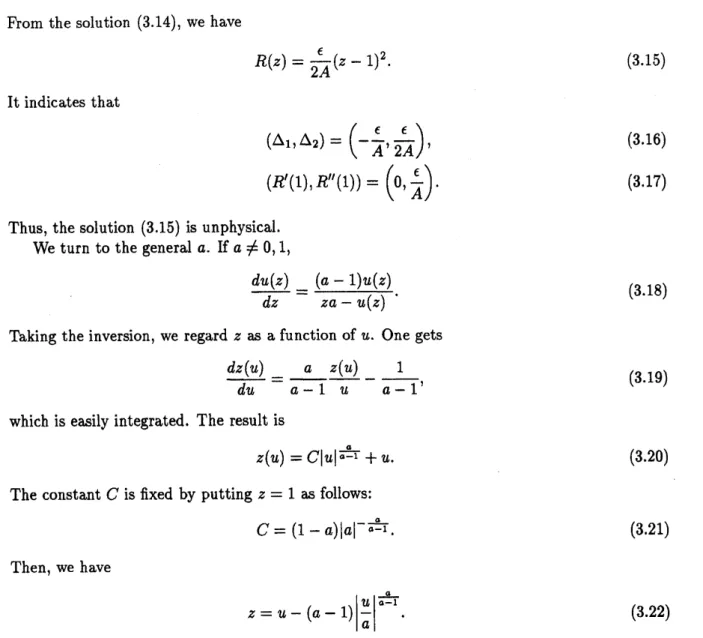
(4.11)

This condition on $\lambda$ implies the existence of slightly relevant modesatthisanalyticfixed point.

In addition to these modes, we find one relevant mode for $v(1)\neq 0$ with $\lambda=1$ by solving

the eigenvalue equation, as well as in the large $N$ limit. This fixed point yielding dimensional

point generally. The only stable fixed point is the trivial fixed point. In a limited coupling

constant space where $R”(1)$ is finite, however, the analytic fixed point is singly unstable in the

following reason. The renormalization groupflow for the couplings $R’(1)$ and $R”(1)$ is depicted

in Fig.4.1. From Fig. 4.1, we find that, for a small initial value of $R$“(1), the flow of $R”(1)$

stays in a compact area. If $R’(1)$ takes a critical value, the coupling $R(z)$ flows toward the

analytic fixed point with a finite $R”(1)$

.

Then, the flow does not generate the relevant mode

with an exponent $0<\lambda<2/N$ from an initial function with afinite $R’$“(1). This analytic fixed

point controls the phase transition, and therefore the critical behavior obeys the dimensional

reduction. Since this analytic fixed point exists for $N\geq 18$ as pointed out by Fisher [2], the

dimensional reduction

occurs

for $N\geq 18$

.

In this case, the critical exponents of correlation

function are given by (2.32). This result agreeswith oursimple $1/N$ expansion [8].

Figure 4.1: The renormalization groupflowfor the couplings $R’(1)$ and $R”(1)$

.

Here we comment on the infinitely many relevant modes pointed out by Fisher [2]. They

are included in the following series inour solution (4.10):

$\alpha_{-}=1-k,$ $(k=3,4,5, \ldots)$ and $C_{+}=0$

.

These belong tothe eigenvalues

$\lambda_{k}=1-k+\frac{2k^{2}}{N}+\mathrm{O}(\frac{1}{N^{2}})$ ,

which

are

positive for sufficiently large $k$

.

These agree with theeigenvalues obtained by Fisher,

although

we

should add aterm $2nkP_{2}P_{k}$ missed in Eq. (C6) of his paper. Since these relevant

modes diverge at $z=-1$

,

we have eliminated them as unphysical modes, as

discussed

above.

5

Conclusion

In thisnote, we have studied the critical phenomena of $(4+\epsilon)$-dimensional random field $\mathrm{O}(N)$

spin model for sufficiently large $N$, by means of the renormalization group method. We find

all fixed points which consist of analytic and nonanalytic ones in the large $N$ limit. On the

other hand for $N<18$, it is known that there are no nontrivial analytic fixed points [2]. By

solving the eigenvalue problem for the infinitesimal deviation from the fixed point, we find

that the nonanalytic fixed points are fully unstable. We search for consistent solutions of the

renormalization

group

with the $1/N$ expansion. If the initial $R”(1)$ is finite, the nonanalytic

relevant modes cannot be generated. In this case, the unique analytic fixed point practically

behaves

as

a singly unstable fixed point, which gives the dimensional reduction. This result

agrees with the stability ofthe replica-symmetric saddle-point solution in the $1/N$ expansion.

Our result also agrees with a recent study of the random field $\mathrm{O}(N)$ model by Tarjus and

Tissier. They study the model by a nonperturbative renormalization group [4]. Although their

work to obtain a full solution is in progress, they give a global picture in a d-N phasediagram

and discuss the consistency of their results with those by some perturbative results. They

propose a scheme to fix aphase boundary ofthe phase where the dimensional reduction breaks

down. Using an approximation method, they show that the phase is in a compact areaon the

d-N plane.

Acknowledgment$\mathrm{s}$

Wewould liketo thank theorganizersoftheRIMS 2005 Symposium, Applications

_of

Renor-malization Group Methods in Mathematical Sciences, held in Kyoto University for giving an

opportunity to talk.

References

[1] G. Parisi and N. Sourlas, Phys. Rev. Lett. 43 (1979) 744-745.

[2] D. S. Fisher, Phys. Rev. B31 (1985)

7233-7251.

[3] M. M\’ezard and A. P. Young, Europhys. Lett. 18 (1992)

653-659.

[4] G. Tarjus and M. Tissier, Phys. Rev. Lett. 93 (2004)

267008-1-4.

[5] J. Z. Imbrie, Phys. Rev. Lett. 53 (1984) 1747-1750; Commun. Math. Phys. 98 (1985)

145-176.

[6] J. Bricmont and A. Kupiainen, Phys. Rev. Lett. 59 (1987) 1829-1832; Commun. Math.Phys.

116 (1988) 539-572.

[7] M. Aizenman and J. Wehr, Phys. Rev. Lett. 62 (1989) 2503-2506.

[8] Y. Sakamoto, H. Mukaida and C. Itoi, Phys. Rev. B72 (2005) 144405-1-18.

[9] A. M. Polyakov, Phys. Lett. B59,79 (1975); Gauge Fields andStrings (Harwood Academic

Publishers, Chur, 1987).

[10] D. E. Feldman, Phys. Rev. Lett. 88, 177202 (2002).

[11] L. Balents and D. S. Fisher, Phys. Rev. B48, 5949 (1993).