Complex dynamics and quantum tunneling in the presence of chaos(New Trends and Applications of Complex Asymptotic Analysis : around dynamical systems, summability, continued fractions)

Complex dynamics

and quantum tunneling

in

the

presence

of chaos

Akira

Shudo

首藤啓 (首都大学東京物理)

Department

_of

Physics, Tokyo Metropolitan University,

1-1 Minami-Ohsawa, Hachioji, Tokyo 192-OS97, Japan

[email protected]

1

Introduction

‘TUnneling phenomenon is peculiar to quantum mechanics and

no

counterparts exist

in classical mechanics. Features of tunneling

are

nevertheless strongly influenced by

underlying classical dynamics [1, 2, 3, 4, 5].

One

of the

most

efficient methods to

analyze quantum tunneling processes is the WKB

or semiclassical

method in which

the classicalorbits

are

employed

as

inputs of approximation. However, since quantum

tunneling is

an

essentially classically forbidden process, real classical orbits have

no

ability to describe it, instead the complex classical orbits play central roles.

It should be recalled that using complexorbits itselfisnot

new

inthe WKBtheory,

rather it

goes

back to the beginning ofthe WKB theory, especially

a text

book

exam-ple of quantum tunneling in

one

dimension. Also,

a

well-known technique using the

complexspaceisthe so-calledinstantonmethod inwhich tunneling penetration

is

eval-uated by a classical path moving along the imaginary time [6]. A natural extension to

higher-dimensional systems wouldbepossible to

a

certain extent aslongasthe system

is completely integrable $[7, 8]$

.

Complexified tori can bridge classically disconnected

regions and

a

semiclassical argument

can

be developed

on

them. However, entirely

different situations

emerge

even

when

one

performs analogous extension tothe system

slightly perturbed from intergrable systems. This is because complexified tori

are

de-stroyed

no

matter how small the strengthof perturbation is and the natural boundary

may appear in complex plane.

2

Time-domain

Semiclassical

Analysis

First,

we

brieflysketchhow

one

can

describequantumtunneling using thesemiclassical

technique.

Dynamical Tunnelng

The system

we are

concerned with is the area-preserving map:

$F$ : _{$\mapsto(q+H’(p)-V’(q)H’(p)-V’(q))$}

.

(1)

Qualitativefeature ofphasespace $(q,p)$ is controlledbythechoice of kinetic term$H(p)$

and also the potential term $V(q)$

.

数理解析研究所講究録

In generic cases, phase space is composed of quatiperiodic regions (2) and chaotic

regions $(C)$, and theseare invariant objects in themselves and disconnectedbyany

clas-sical orbits. However, in quantum mechanics, the tunnelingeffect allows the transition

between two any disconnected components of

₂

and $C$, and quantum tunneling

over

such dynamical barrierss is particularly called dynamical tunneling in the literature.

More precise specification

or

definition of quantum tunneling in the present setting is

provided later,

Quantum Propagator

A standard recipe to construct quantum mechanics of the area-preserving map is first

to express unitary operator in the discretized Feynman path integral form. In the

momentum (p-) representation, for example, the$n$-step quantum propagator is written

as

$K(p_{0};p_{n})=<p_{n}|U^{n}|p_{0}>= \int\cdots\int\prod_{j}dq_{j}\prod_{j}dp_{j}\exp[\frac{i}{\hslash}S(\{q_{j}\}, \{p_{j}\})]$, (2)

where $S(\{q_{j}\}, \{p_{j}\})$ denotes the discretized action along each path The classical map

(1) is recovered by imposing the variational condition $\delta S(\{q_{j}\}, \{p_{j}\})=0$.

SemiclassicalApproximation

In order to include the complex orbits that

are

inevitable to describe classically

for-bidden processes, instead of applying the stationary phase method,

we

evaluate the

quantum propagator $<p_{n}|\hat{U}^{n}|p_{0}>\mathrm{b}\mathrm{y}$ the saddle point method. Thefinal expression

for the semiclassical propagator inp–representationtakes the form as

$K^{\epsilon c}(p_{0};p_{n})= \sum_{\gamma}A_{\gamma}(p_{0},p_{n})\exp\{\frac{i}{\hslash}S_{\gamma}(p_{0},p_{n})\}$

,

(3)

$\mathrm{f}\mathrm{i}\mathrm{n}\mathrm{a}1\mathrm{m}\mathrm{o}\mathrm{m}\mathrm{e}\mathrm{n}\mathrm{t}\mathrm{a},p_{0}=\alpha \mathrm{a}\mathrm{n}\mathrm{d}p_{n}=\beta A_{\gamma}(\mathrm{p}0,p_{n})=[2\pi\hslash(\partial p_{n}/\partial q\mathrm{o})_{p0}]^{-}\mathrm{W}\mathrm{h}\mathrm{e}\mathrm{r}\mathrm{e}\mathrm{t}\mathrm{h}\mathrm{e}\mathrm{s}\mathrm{u}\mathrm{m}\mathrm{m}\mathrm{a}\mathrm{t}\mathrm{i}\mathrm{o}\mathrm{n}\mathrm{i}\mathrm{s}\mathrm{t}\mathrm{a}\mathrm{k}\mathrm{e}\mathrm{n}\mathrm{o}\mathrm{v}\mathrm{e}\mathrm{r}$

.

$\mathrm{a}11\mathrm{c}1\mathrm{a}\mathrm{s}\mathrm{s}\mathrm{i}\mathrm{c}\mathrm{a}1\mathrm{p}\mathrm{a}\mathrm{t}\mathrm{h}\mathrm{s}\gamma \mathrm{s}\mathrm{a}\mathrm{t}\mathrm{i}\mathrm{s}y\mathrm{i}\mathrm{n}\mathrm{g}\mathrm{f}\mathrm{i}_{\overline{2}\mathrm{s}\mathrm{t}\mathrm{a}\mathrm{n}\mathrm{d}\mathrm{s}\mathrm{f}\mathrm{o}\mathrm{r}\mathrm{t}\mathrm{h}\mathrm{e}}^{\mathrm{i}\mathrm{v}\mathrm{e}\mathrm{n}\mathrm{i}\mathrm{n}\mathrm{i}\mathrm{t}\mathrm{i}\mathrm{a}1\mathrm{a}\mathrm{n}\mathrm{d}}$

amplitude factor

as

sociated with the stability of each orbit 7, and $S_{\gamma}(p_{0},p_{n})$ is the

corresponding classical action.

Initial Value Representation

The semiclassical

sum

(3) contains not only real classical orbits but also complex

clas-sical ones, the latters would be responsible for the tunneling process. One physical

requirement is that since

we

take thep–representation, $p_{0}$ and$p_{n}$ should be real-valued

since they both

are

observables. This implies that

a

canonical conjugate variable $q_{0}$

does not have any constraint and

may

take not only real values but also complex ones,

so

itinerary from $(p_{0}, q_{0})$ to $(p_{n}, q_{n})$ may be complex. To include complex orbits,

we

extend the initial angle

as

$q0=\xi+i\eta$ $(\xi, \eta\in \mathbb{R})$

.

For given $\alpha,$$\beta\in \mathbb{R}$,

we

have

a

representationfor semiclassically contributing complex paths

as

Mg,

$\beta_{\equiv\{(p_{0},q_{0}=\xi+i\eta)\in \mathbb{C}^{2}}|p_{0}=\alpha,$ $p_{n}=\beta$

}.

(4)

If there exist no classical orbits on the realphase space connecting two states $p_{0}=\alpha$

and$p_{n}=\beta$,

we

should say that this process is classically forbidden, and bridged only

3

Tunneling

Orbits

in

the

Linear map

Before going to chaotic maps,

we

examine the linear map. The linear map is helpful

to

understand

what

classical

objects represent quantum tunneling and to know what

are new

ingredients in chaotic maps.

Solutions

The linear map is given

as

$F:\mapsto$

, (5)

where $\omega$ is

a

fixed rotation number. It is easy to show that $(p_{n}, q_{n})$

are

expressed by

$(p_{0}, q_{0})$

as

$p_{n}=p_{0}+K_{n}\sin(q_{0}+n\omega/2)$ ,

$q_{n}=q_{0}+n\omega$,

where $K_{n}=K \sin(n\omega/2)/\sin\frac{(d}{2}$

.

For

a

given initial condition $p_{0}=\alpha\in \mathbb{R}$, in order to

have $q_{n}\in \mathbb{R}$ the initial coordinate $q_{0}=\xi+i\eta$ should satisfy

$\xi=(k+\frac{1}{2})\pi-\frac{n\omega}{2}$ ($k$ : integer)

or

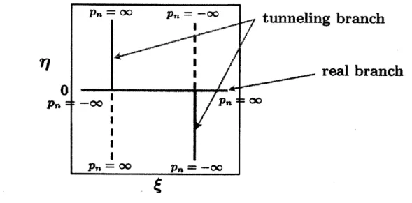
_$\eta=0$. (6)

Tunneling Branches

Figure 1 illustrates

a

set ofinitial conditions that contribute to the semiclassical

sum

(3)

$\mathcal{M}_{n}^{\alpha,*}=\{q_{0}=\xi+i\eta|p_{0}=\alpha, -\infty<p_{n}<\infty\}$. (7)

Here

we

set $\alpha=0$

.

The orbits satisfying the former condition in (6)

are

real orbits,

and the latter

are

complex

ones.

Note that tunielingbranches appear in apair-wise

manner as

shown in Fig. 1; the

one

givingexponentially decayingandthe other exponentially blowing upcontribution.

The former is a correct tunneling branch and the latter is unphysical and should be

removed

as a

result of

Stokes

phenomenon. TheStokes phenomenon is quite important

in the complex WKB analysis, however, we do not discuss this issue here. (See [9] for

example.)

Figure (2) is a schematic sketch demonstrating that pairs of tunneling branches

emanating from the real Lagrangian manifold. Note that tunneling tails in the

wave-function

are

reproducedby tunnelingbranches.

An

importantremarkis that, in order to go into deep tunnelingregions,

one

should

take

a

large ${\rm Im} q_{0}=\eta$

.

That is, the amount of imaginary part necessary to allow the

tunneling transition is gained in the imaginary part of the initial condition. We

can

say, otherwise, that

no

dynamics is involvedin the tunnelingprocess oflinear map and

only the initial condition controls it. It is worthwhile to note that ${\rm Im} q0=\eta$ play

an

analogous role of imaginary time that is used in the so-called instanton method [6].

The instanton orbit

runs

in the imaginary direction in complex time domain, and the

higher potential barriers

one

wants to go beyond, the deeper imaginary time domain

one has to

use.

Figure 1: The initial valueplaneintroducedas (7). The lines running in the vertical direction

give thetunneling contributions.

4

Tunneling Orbits

in

Ideally

Chaotic Maps

In contrast to the previous one, tunneling orbits in chaotic maps behave quite

differ-ently. We first

see

how tunneling orbits

appear

in the most generic situations, mixed

systems.

hnneling Orbits in The Standard Map

There

are a

varietyof chaotic mapsin theform (1) thatrealize mixed-type phase space.

We here consider the standard map: $H(p)=p^{2}/2,$ $V(q)=K\sin q$

.

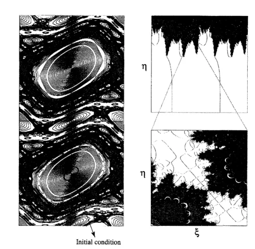
Figure 3 shows

a

typical mixed phase space with

some

moderate parameter value and the corresponding

initial value set $\mathcal{M}_{n}^{\alpha,*}$

.

In the semiclassical propagator, the initial state is taken as

an

ellipse approximating

a

KAM curve, not$p_{0}=const$as in the linear map. In the initial

set $\mathcal{M}_{n}^{\alpha,*}$, two

curves

running in the vertical direction that exactly corresponds to the

tunneling branches shown in Fig. 1. The mechanism of tunneling induced by such

branches

are

essentially the

same

as

the

one

taking place in the linear

map.

However,

in case

of

the standard map, there are a huge number of branches

not

touching

on

the

real axis, $\eta=0$

.

Allthese

are

due to that the system is not completely integrable and

the map generates chaos not only inreal but also in complex plane.

We skip all the details concerning the mechanism creating tunneling tails in

quan-tum wavefunctions [4]. Ofsignificantly importance isthatspecific sequencesofbranches,

which, as shown in Fig. 3, usually form successive chain-like structures, control the

tunneling processes, meaning that we have only to focus

on

these specific structures.

We remark that the existence ofthese chained objects is not limited to the standard

map.

The H\’enon Map

polyno-Figure 2: (a) The real Lagrangian manifold and tunnelingbranches. An exact form of the

real Lagrangian manifold is expressed as$p_{n}=p_{0}+K_{n}\sin(q_{n}-n\omega/2)$

.

$(\mathrm{b})$ The wavefunction

inthe p- representation (schematic). (c) Thereal Lagrangian manifold and pairsoftunneling

branches (schematic).

mial functions. There

are

several

reasons

to employ theH\’enon map: the most relevant

one

is that complex dynamics has been and is being most extensively investigated,

a

part of which is introduced below. This is important because the understanding of

what is going on in complex phase space is crucial.

A canonical form of the H\’enon map is given as $f$ : $(x, y)\mapsto(y, y^{2}-x+a)$, but

an

alternative form obtained by

an

affine change of variables

as

$(p, q)=(y-x, x-1)$

together with

a

parameter $c=1-a$

fits

the present

purpose:

$F:-\rangle$

, $V(q)=- \frac{q^{3}}{3}-cq$. ₍₈₎

The H\’enon map has

a

nonlinear paremeter $a$ (or $c$) controlling the dynamics

qualita-tively. When $a\gg 1$_, the so-called horseshoe condition is satisfied and the mapping is

conjugate to the symbolic dynamics with the binary full shift [10]. All the stable and

unstablemanifolds intersect transversally when thehorsehoe is realized and the system

keepshyperbolicity uptothe first tangencypoint [11]. Non-wondering set formsfractal

repeller on the real plane.

Figure 3: (a) Phase space for standard map with $K=1.5$. An ellipse in the lower torus

region is the initial condition. (b) The initial value set $\mathcal{M}_{n}^{\alpha,*}$ at $n=6$ and its magnification.

The Horseshoe Limit: An Ideal Setting

The horseshoe limit provides

an

ideal situation where the chained structure observed

in generic

case

appears in a genuine

manner.

Figure 4 demonstrates the set $\mathcal{M}_{n}^{\alpha,*}$ when the parameter $c$ is within the horseshoe

locus. We notice that

a

similar chained structure

as

found in Fig. 3 is formed. A

relation between $\mathcal{M}_{n}^{\alpha,*}$ and invariant objects in dynamical systems is read by putting

the intersection of the (complex) stable manifold $W^{\mathit{8}}(p)$ of periodic orbits _$p$ with the

initialvalue plane$\mathcal{I}=\{(q,p)\in \mathbb{C}^{2}|p_{0}=\alpha\}$. The intersection points

are

alignedalong

the chain and the labels inserted in the figure denote the binary coding for periodic

orbits from where the stable manifolds $W^{s}(p)$ emanate. That is, for example, the dot

labeled

as

(000) is

a

point at which the stable manifold of the periodic orbit whose

binary coding is (000) intersects with the initial value plane $\mathcal{I}$

.

Recall that, in the

horseshoe parameter locus, all the periodic orbits

are

contained in $\mathbb{R}^{2}$

. The chained

structure is associated withinvariant structures in phase spacein thisway.

As a

result,

the itineracy of the orbits launched

on

the chained structure is governed by the stable

manifold attached to it. As shown in Fig. 4(b), the orbits whose initial conditions

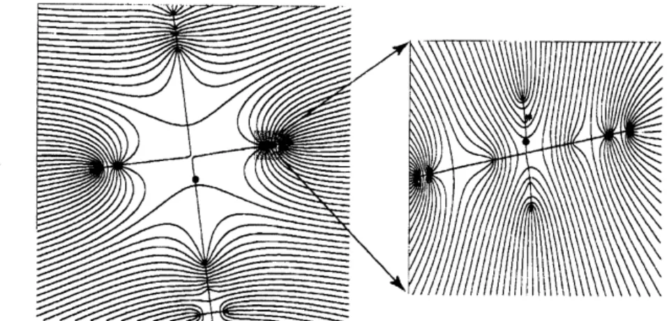
Figure 4: (a) The initial value set $\mathcal{M}_{n}^{\alpha,*}$ at $n=3$ for the H\’enon map in the horseshoe

parameter locus. The dots representthe primary intersection points (see thedefinition in the

text) of(complex) stable manifolds and the initial value planeT. (b) The distance from the

real plane as afunction of the time step $n$

.

The orbits arelaunched from the pointson$\mathcal{M}_{n}^{\alpha*}$)

and close to the intersectionpoints.

orbitsclosely followthe orbits

on

the stable manifolds.

Otherwise

stated, thetunneling

orbits forming chained structures

are

guided by the stable manifolds of the periodic

orbits [12]. In

a

similar manner,

on

the chained structure found in generic mixed

case

(Fig. 3), the orbits startingfrom it also approachesthe real plane exponentially.

Other

orbits, not forming the chain, do not shows such behavior and

are

not attracted from

the real plane.

Tree Structure in Hyperbolic Case

It is instructive to

see

the situation where the system is hyperbolic but not in the

horseshoe locus. Such a situation may not be

so common.

For instance, in the

stan-dard

map,

except for the so-called anti-integrable limit, phase space is composed of

quasiperiodic and chaotic components. In the H\’enon map, there indeed exist

param-eter loci in which the dynamics

on

the real plane is hyperbolic but cannot be reduced

to the binaryfull shift asthe horseshoelimit does

so.

The existence of such parameter

loci

was

suggested in [14], and recently shown rigorously via computer-assisted proof

[15].

The

reason

why hyperbolic but not horseshoe

cases

are so

important in

our

issue is

thatit can be amodel to examine how tunneling orbitsbehavewhenthe non-wondering

set is

no

more

confined onthe real plane, and therebyreal andcomplex saddlescoexist.

In the horseshoe locus,

as

depicted in Fig. 4, each chain

runs

only in the vertial

direction. However,

as

seen

in Fig. 5, the tree structure begins to develop in $\mathcal{M}_{n}^{\alpha,*}$

. Furthermore, though not shown here,

as

the time step proceeds,

we can see

that

the number

of

generation increases.

Here

we use

the term generation

as

a

rank in the

hierarchicaltree structures. The chained branch runningin theperpendiculardirection

is the

first

generation and horizontal

one

the second generation and

so on.

Figure

5:

(a) The initial value set $\mathcal{M}_{n}^{\alpha,*}$ at $n=20$ for the H\’enon map in the parameter

locus at which the map is hyperbolic but not has the horseshoe structure. The dots shown

are some of primary intersection points _{of (complex) stable manifolds and the initial value}

plane Z. The right hand figure isa magnification of the left one.

Primary Intersection Points

To explain the implication ofthe tree structure,

we

introduce the ordering for

inter-section points ofstable manifolds and the initial value plane Z.

Here, theprimary intersection is defined as anintersectionpoint atwhich the stable

manifold $W^{s}(p)$ emanating from a saddle _$p$ (period $n$) first intersects with Z. More

precisely, we specify the ordering of the intersection

as

follows: it is known that there

is

a

conjugation map $\Phi$ from $\mathbb{C}$ to _$W^{s}(p)$ such that

$\Phi^{-1}F^{n}\Phi=F_{\epsilon n}$ where $F_{sn}(\zeta)=\lambda^{-1}\zeta$ (9)

for

$\zeta\in$

C.

Here

A denotes

the maximal eigenvalue of the tangent map of $F^{n}$ at _$p$

.

The coordinate $\zeta$ is normalized in the

sense

that the map $F^{n}$ is expressed by

a

linear

transformation. Putting

an

appropriate domain, say$D$ on the $\zeta$-plane, containing

$p$

as

the origin of $\zeta$-plane and $D’=D-F_{sn}(D)$, the $\zeta$ plane is decomposed into

a

family

ofdisjoint domains $D_{m}=F_{sn}^{-m}(D’)(m\in \mathrm{Z})$

.

Here, the primary intersection is defined

as an intersection point between $\mathcal{I}$ and _$W^{s}(p)$ in

$D_{m}$ with the minimal $m$ in the $\zeta$

coordinate.

The dots shown in Fig.

5

are some

of primary intersection points

so

defined. As in

the horseshoe case, each intersectionpoint is attached to

a

curve

of$\mathcal{M}_{n}^{\alpha,*}$

.

In contrast

to the horseshoe case, however, the orbits launched at points

on

the tree-shaped $\mathcal{M}_{n’}^{\alpha}$“

do not approach the real plane monotonically. To

see

the difference,

we

observe the

behavior

of the orbits whose initial conditions

are

close to the primary intersection

points. We plot in Fig. 6(a) the distance from the real plane

as a

function of time

step $n$ and the corresponding schematic representationof the set $M_{n}^{\alpha,*}$ is given

as

Fig.

Figure 6: (a) The distance from the real plane as afunction of time step $n$

.

Theorbits are

launched from the points on $\mathcal{M}_{n}^{\alpha,*}$ and close to the primary intersection points in the tree

structure. (b) Tree structure and the primaryintersection points (schematic).

Itineracy in The Complex Phase Space

For the interpretationofthe originofthe behavior observed in Fig. 6(a), the following

theorem is crucial:

$\mathrm{T}\mathrm{h}\mathrm{e}\mathrm{o}\mathrm{r}\mathrm{e}\mathrm{m}$[$\mathrm{B}\mathrm{e}\mathrm{d}\mathrm{f}\mathrm{o}\mathrm{r}\mathrm{d}$-Smillie] For any saddle

$p,$ $\overline{W^{\epsilon}(p)}=J^{+}$ and also$\overline{W^{u}(p)}=J^{-}$

Here $J^{\pm}=\partial K^{\pm}$ and $K^{\pm}=$

{

$(p,$$q)|$ $||F^{n}(p,$ $q)||$ is bounded $(narrow\pm\infty)$

}.

Since

$K^{\pm}=J^{\pm}$ in the hyperbolic case, the above theorem claims that any stable

manifold

is dense in the forward bounded orbits $K^{+}$

.

Now, let $\mathrm{r}_{i}$ and

$\mathrm{c}_{j}$ be the

saddles

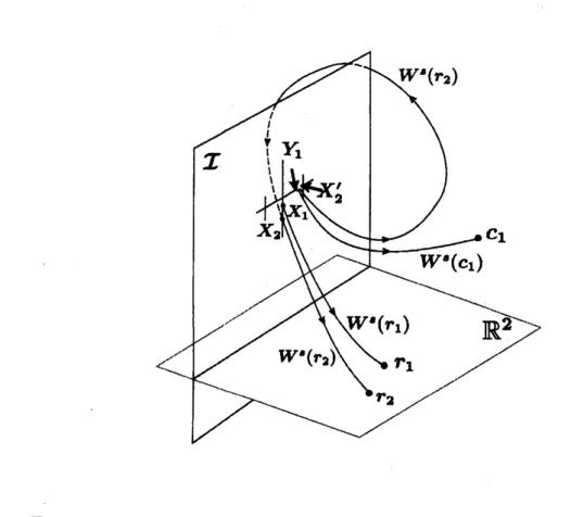
in the real and complex plane, respctively. We

then introduce the primary intersections between $\mathcal{I}$ and $W^{\epsilon}$ of these two kinds of

saddles, say $\mathrm{r}_{1}$ and $\mathrm{c}_{1;}$ they

are

denoted by $\mathrm{X}_{1}$($\in W^{\epsilon}(\mathrm{r}_{1})$ fiZ) and $\mathrm{Y}_{1}(\in W^{\delta}(\mathrm{c}_{1})\cap \mathcal{I})$,

respectively (see Fig. 7).

Consider

a

side branch in the second genetation, which is attached to the

intersec-tion pointdenotedby$\mathrm{Y}_{1}=W^{s}(\mathrm{c}_{1})\cap \mathcal{I}$

.

Since$\mathrm{Y}_{1}$ islocated close to$\mathrm{X}_{1}$, the trajectories

starting at $\mathrm{X}_{1}$ and $\mathrm{Y}_{1}$ trace similar itinerary in the very initial time stage. But the

orbit launched at the $\mathrm{Y}_{1}$ finally approaches $\mathrm{c}_{1}$ by definition and cannot reach the real

phase space. However, the fact $\overline{W^{s}(p)}=J^{+}$ implies that in a very close neighborhood

of $\mathrm{Y}_{1}$ there exists

an

intersection $\mathrm{X}_{2}’\in W^{\epsilon}(\mathrm{r}_{2})\cap \mathcal{I}$ of

a

real saddle $\mathrm{r}_{2}(\mathrm{r}_{2}$

can

be $\mathrm{r}_{1})$. Let the primary intersectionof$W^{s}(\mathrm{r}_{2})$ and $\mathcal{I}$be $\mathrm{X}_{2}$, then the trajectory from$\mathrm{X}_{2}$

converges

directly to $\mathrm{r}_{2}$, whereas the trajectory from $\mathrm{X}_{2}’$ first approaches

$\mathrm{c}_{1}$ because

$\mathrm{X}_{2}’$ is

very

close to$\mathrm{Y}_{1}=W^{s}(\mathrm{c}_{1})\cap \mathcal{I}$ and next

converge

to $\mathrm{r}_{2}$, which

means

that $\mathrm{X}_{2}’$ is

the secondary intersection of $W^{\epsilon}(\mathrm{r}_{2})$ with $\mathcal{I}$

.

In other words, the trajectory from

$\mathrm{X}_{2}’$

makes

a

side trip in the complexdomain before accessing to the real plane.

In the same way, there should exist $\mathrm{Y}_{2}’=W^{\epsilon}(\mathrm{c}_{2})\cap \mathcal{I}$ which is located just at the

side of

_X’2’

where $\mathrm{c}_{2}$ denotes another complex saddle. The side chain of thethird order

is realized very close to the tirtiary intersection $\mathrm{X}_{3}’’$ of the intersction $\mathcal{I}\cap W^{s}(\mathrm{r}_{3})$, if

$n$ is taken large enough. Inductively, the m-th order generation, germinates from the

$(m-1)$-th order generation.

Figure 7: Initial valueplane$\mathcal{I}$ and stable manifolds for real saddles (schematic).

As predicted by the theorem $\overline{W^{\partial}(p)}=J^{+}$ and numerical observations imply that

there

exist

a

rich variety of tunnelingpathswandering

over

complex phase

space

before

reaching close to the real plane. Ishii gave a rigorous statement supporting such

an

aspect [12]. It

assures

the existence of orbits that allow trajectories exhibiting chaotic

itinerancy

over

the complex saddles:

Theorem[Ishii] Let $0<h_{\mathrm{t}\mathrm{o}\mathrm{p}}(F|_{\mathrm{R}^{2}})<\log 2$ and let$p_{i}(1\leq i\leq N)$ be saddle periodic

points in $\mathbb{C}^{2}\backslash \mathbb{R}^{2}$

.

Take any positive integers $k_{i}$ and any neighborhood $U_{i}$

of

$p:(1\leq$

$i\leq N)$. Then, there exists a point $z\in \mathbb{C}^{2}\backslash \mathbb{R}^{2}$ such that its orbit stays in $U_{i}$ at least $k_{i}$-times iterates and _{$\lim_{narrow\infty}d(F^{n}(z), \mathbb{R}^{2})=0$}

.

Theconvergenttheorem ofcurrents is

a

central result ofBedford and Smillie andmany

resultsfollow from it [17, 16, 18]. The above theorem essentially

uses

theresults of[18].

An

importantfactis,

as

mentionedbelow, that the convergent theoremapplies notonly

to hyperbolic but also to anycasesincludingmixedphasespace. Therefore, it isnatural

to expect that the behavior just sketched above is not limited to the hyperbolic case.

In fact, the orbits

launched

at a chained branch in the higher generation, for example

Why Are Chained Structures So $Important^{Q}$

Up tonow, we only

saw

the behavior of complex orbits that contribute to the

semiclas-sicalpropagator (3). The readers may have questions

as

towhy thechained structures

found commonly in the initial value plane is so important in

our

tunneling problem.

We have entirely skipped this topic.

Themain

reason

is that,

as

shownin Fig. 4, the orbits forming the chain structure

approach the real plane exponentially. Correspondingly, the imaginary part of action,

${\rm Im} S_{n}$,

converges

rapidly and

we may

expect that $|{\rm Im} S_{n}|$ takes the smallest values

as

comparedwith those forthe orbits taking side trip, unless

some

nontrivial cancellation

mechanism works initinerating

orbits.

Since

theweightofeach term in the semiclassical

sum

(3) is almost controlled by${\rm Im} S_{n}$, the orbits that gain the minimal ${\rm Im} S_{n}$

are

most

dominantcontributors inthe

sum.

This is

a

rough reasoning for theimportance of the

chainedobjects. Itis not yetclearthat theorbitswondering in complex

space, as

found

in Fig. 6(a), play

some

roles in the tunneling problem. If they make non-negligible

contributions,

we

may say that genuine complex chaos appears in quantum tunneling.

More detailed aruguemts of observability ofcomplex chaos in quantum tunneling will

be discussed in [13].

5

Tunneling

Orbits

in Mixed Phase Space

Initial andFinal

_Manifolds

in Semiclassical Dynamics

As

often emhpasized, the most natural and important situation is that KAM

curves

and chaotic regions coexist in phase space. That is, the transition from KAM regions

to chaotic seas has particularly to beinvestigated. To focus ourproblem

more

sharply,

we again make clear the setting of the semiclassical argument.

So far,

we

have taken$\Psi$-representation like eq. (2). However,

we can

freely replace

it to other representations. For example,

we

may take the coherent representation

$K(q_{n},p_{n};q_{0},p_{0})=<q_{n},p_{n}|\hat{U}^{n}|q_{0},p_{0}>$. Here $|q,p>=|a>\mathrm{d}\mathrm{e}\mathrm{n}\mathrm{o}\mathrm{t}\mathrm{e}\mathrm{s}$the coherent state

with $a=(q+ip)/\sqrt{2}$

.

We have a similar semiclassical _expression

as

$K^{sc}(q_{n},p_{n};q_{0},p_{0})= \sum_{\gamma}A_{\gamma}(p_{0}, q_{0})\exp\{\frac{i}{\hslash}S_{\gamma}(p_{0}, q_{0})\}$ , (10)

wherethe sumis taken

over

allclassical pathssatisfyinggiven initial andfinal coherent

states, $i.e.,$ $q0+ip_{0}=q_{\alpha}+ip_{\alpha},$ $q_{n}-ip_{n}=q_{\beta}+ip_{\beta}$

.

Notethat thevariables$q_{\alpha},p_{\alpha},$$q_{\beta},p_{\beta}$

take real values whereas $q_{0},p0,$$q_{0},p_{0}$ can take complex ones $[19, 20]$

.

Introducing the

variables $Q=q+ip$ and $P=q– ip$ where $q,p\in \mathbb{C}$, semiclassically contributing

complex paths

are

given

as

$M_{n}^{\alpha,\beta}\equiv\{(Q_{0}, P_{0})\in \mathbb{C}^{2}|Q_{0}=\alpha, P_{n}=\beta, \alpha=q_{\alpha}+ip_{\alpha}, \beta=q_{\beta}-ip_{\beta}, \}$

.

(11)

Note

thatin

any

representation the manifold of initial

or

final

states

is

one-dimensional

complex manifold, thereby the space of the search parameter forms one-dimensional

complex plane. This is interpreted

as a

manifestation ofuncertainty principle of

quan-tum mechanics.

Convergent Theorem and Mixing Property in Complex Phase Space

The semiclassical dynamics is therefore just to follow the time evolution of a

one-dimensional complex manifold with a boundary condition imposed on the final state.

The finalstate is also expressed

as

one-dimensional complex manifold. We again recall

that the asymptotic behavior ofwide classes ofmanifoldsis wellcontrolledusing

poten-tially

theoretic

arguments

of

complex dynamical systems [17, 16, 18], More precisely,

the following convergent theorem

_of

currents tells

us

how one-dimensional manifold

behaves asymptotically: Theorem[Bedford-Smillie]

For

a

complex one-dimensional locally closed

_sub-manifold

$M$ in either $J^{\pm}$ or an

alge-braic variety, there is a constant$\gamma>0$

so

that

$\lim_{narrow+\infty}\frac{1}{2^{n}}[F^{\mp n}M]=\gamma\cdot dd^{c}G^{\pm}(x, y)$ (12)

in the

sense

_of

current, where $[M]$ is the current

of

integration

of

$M$, i.e. $[M](\phi)\equiv$

$\int_{M}\phi|_{M}$

.

In this statement, $G^{\pm}(x, y)$ represents the

Green

function

given by

$G^{\pm}(x, y) \equiv\lim_{narrow\pm\infty}\frac{1}{2^{n}}\log^{+}||F^{n}(x, y)||$, (13)

where $dd^{c}$ is the complex Laplacian,

$dd^{\mathrm{c}}u \equiv 2i\sum_{j,k}\frac{\partial u}{\partial z_{j}\partial\overline{z}_{k}}dz_{j}\wedge d\overline{z}_{k}$ (14)

The statement claims that

an

arbitrary algebraic curve in $\mathbb{C}^{2}$, for example

our

initial

manifold given

as

$p_{0}=\alpha\in \mathbb{R}$, converges to the $\mathrm{s}\mathrm{u}\mathrm{p}\mathrm{p}o\mathrm{r}\mathrm{t}$of$dd^{c}G^{\pm}(x, y)$

.

Moreover,

$\mathrm{T}\mathrm{h}\mathrm{e}\mathrm{o}\mathrm{r}\mathrm{e}\mathrm{m}$[$\mathrm{B}\mathrm{e}\mathrm{d}\mathrm{f}\mathrm{o}\mathrm{r}\mathrm{d}$-Smillie]

$\mu$ is mixing and the hyperbolic

measure.

Here $\mu\equiv\mu^{+}\wedge\mu^{-}$ and $\mu^{\pm}$ is

induced

by the Green function

as

$\mu^{\pm}\equiv\frac{1}{2\pi}dd^{c}G^{\pm}(x, y)$

.

(15)

The complex equilibrium

measure

$\mu$ thus defined becomes a unique maximal entropy

probability

measure

[17, 16, 21, 18].

Implications in The Tunneling Problem

Since the asymptotic behavior is

so

described by the convergent theorem,

we

obtain

theorems

on

the relation between tunneling orbits and the Julia set in the

forward

direction

by taking into account the final

states

also [12]. The result indeed supports

and is consistent with numerical

observations

illustrated in Figs. 3, 4, and

6.

In this

sense,

we can

say that, in contrast to tunneling orbits in the linear map, the complex

orbits behind tunneling processes in chaotic systems have truly different characters.

As stressedin section 3, tunneling penetration does not

occur

as a

result

of

dynam-ics in the linear map, but gaining the imaginary part ofthe initial condition makes it

possible.

On

the hand hand, in the H\’enon map, due to the mixing property stated

above, arbitrary neighborhoods of the points in the Julia set are connected by the

the role, the coherent state representation is useful since the coherent state is a

min-imal wavepacket, and is

an

object closes to an orbit in classical dynamics. For any

neighborhood $U_{\alpha}$, $U_{\beta}$ of initial and final points, $(q_{\alpha},p_{\alpha})$ and $(q_{\beta},p_{\beta})$ in the coherent

representation, there exist atime step $N$ such that $f^{N}(U_{\alpha})\cap U_{\beta}\neq\emptyset$

.

Since the

neigh-borhood $U_{\alpha}$ shouldbe taken

as

an open set in $\mathbb{C}^{2}$,

the orbit connectingbetween $U_{\alpha}$ and

$U_{\beta}$

may

not be contained in the initial manifold $\mathcal{M}_{n}^{\alpha,\beta}$. However;

we

can

find another

initial state $(q_{\alpha}’, p_{\alpha}’)$ that

can

be taken arbitrarily close to the original point $(q_{\alpha},p_{\alpha})$

which contains

a

desired orbit. In other words, although

one

cannot

say

that

a

set

$M_{n}^{\alpha,\beta}$ always contains

a

connecting orbit, there is

a

wavepacket arbitrarily close to the

original

one

whose initialplane $\mathcal{M}_{n}^{\alpha’,\beta’}$ containssuch

a

connecting orbit. Thetunneling

transition, reflectingthe mixing property ofthe complexmeasure$\mu$, takes place in this

way.

Complexified $KAM$ Curves and Natural Boundaries

As mentioned, theorems of Bedford and Smillie are suggestive and certainly give

a

fundamentalprinciple forthesemiclassicaldescription of quantum tunneling processes.

However, only to know the existence of invariant

measure

having such nice properties

is not enough to get further predictive view in tunneling phenomena. since the most

important process, that is, the transition from the region dominated by KAM

curves

to chaotic regions, necessarily involves many delicate issues in the problem of nearly

integrable Hamiltonian dynamics,

so

more

precise information

on

complex structures

in such regions is strongly required.

In particular, we need to discuss the role of complexified $KAM$

curves.

To this

end, the works done by several authors who studied the domain ofanalyticity of

com-plexified KAM curves become significant clues $[22, 23]$

.

The aim in those works was

to specify a critical value of the perturbation parameter $K_{c}$ at which the last KAM

circle disappears, and also to study the universality of the critical function $K(\omega)$: the

breakdown threshold ofthe KAM

curve

with rotation number $\omega$. Here we will

see

that

this subject is indeed of fundamental importance in the tunneling problem.

A

standard recipe to consider the analyticity domain of

KAM

curves

is first to

express KAM

curves

parametrically

as

$C_{\omega}$ : _{$=(2\pi\omega+u(\varphi, \omega)-u(\varphi-2\pi\omega, \omega)\varphi+u(\varphi,\omega))$}, (16)

where $u(\varphi, \omega)$ is determined by the following functional equation:

$u(\varphi+2\pi\omega, \omega)-2u(\varphi, \omega)+u(\varphi-2\pi\omega, \omega)=V’(\varphi+u(\varphi,\omega))$. (17)

The dynamics

on

the

curve

$C_{\mathrm{t}d}$ is given in the

$\varphi$-variable as a constant rotation _{$\varphi_{n+1}=$} $\varphi_{n}+2\pi\omega$

.

For

a

givenrotation number $\omega$, the existence of

an

analytic KAM

curve

is

equivalent to the existence of

a

positive radius of

convergency

of the Lindstedt series,

$u( \varphi, \omega)\equiv\sum_{k=1}^{\infty}K^{k}\sum_{\nu\leq k}\mathrm{e}^{i\nu\varphi}u_{\nu}^{(k)}(\omega)$

.

(18)

As first suggested in Ref. [22], making analytical continuation of the Lindstedt series

to the complex plane, one can do it at most to a certain domain of $\varphi$-plane and there

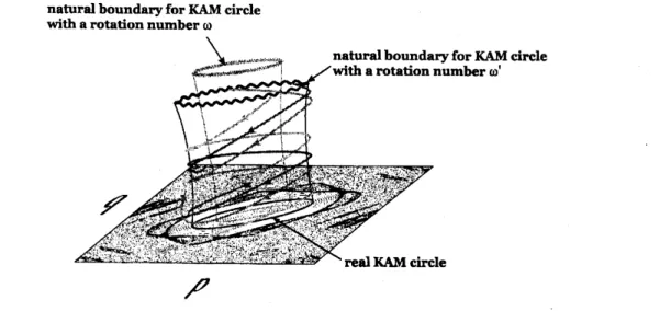
possiblyexist a natural boundary. The existence of the natural boundary implies that

naturalboundary forKAMcircle witharotationnumber$\omega$

$\nearrow$

Figure

8:

Naturalboundaries of KAM circles (schematic). Thecomplexorbits which describe

tunneling processes are also inserted in the figure. Those orbits launched almost around

naturalboundaries and go down to the realplane. Thedistance from the realplane decreases

exponentially, just as shown in Fig. 4(b) and the bold lineofFig. 6(a).

KAM circles cannot be globally invariant in complex plane. Numerical observations

suggest the shape ofthe boundary is fractal in $(q,p)$-plane. Weschematically draw

an

aspect in Fig.

8.

Mixing in the Complexified $KAM$ Regions $l$

?

The orbits on KAM

curves

are bounded both in the forward and backward directions,

so

they

are

contained in the filled-in Julia set $K=K^{+}\cap K^{-}$ Note that numerical

testssuggest that $K^{\pm}$ have no

interior points [9]. There is

no

rigorous proof validating

those numerical results, but if$K^{\pm}$ have no interior points, $J=K$ follows.

Next we ask the relation between $J$ and $J^{*}=\mathrm{s}\mathrm{u}\mathrm{p}\mathrm{p}\mu$. In case the system is

hyper-bolic, $J=J^{*}$ holds, but in general it

was

atmost proved that $J^{*}\subset J$

.

In non-hyperbolic

or

mixed systems, both possibilities remain: (i) $J=J^{*}$ or (ii) $J\neq J^{*}$. If the former

holds, it immediately follows that

_{{KAM curves}}

$\subset J^{*}$. Since the mixing property

holds

on

$J^{*}$,

a

more

specified situation just mentioned above is realized, that is the

mixing property of complex dynamics allows the connection between two separated

regions via the realdynamics.

On

the other hand, if the

case

(ii) is true, it

can

happen

that such orbits do not necessarily exist.

It is not an easy task to check which situation is really the case even numerically.

Whatwehave presented in Fig.

9

isatypicalbehaviorof the orbits sandwiched between

complexified KAM

curves.

Herewe put aninitial point $(q_{0},p_{0})$ such that $({\rm Re} q_{0}, {\rm Re} p_{0})$

is on a certain KAM circle and $|{\rm Im} q_{0}|,$ $|{\rm Im} p_{0}|\ll 1$. The orbit so locatedvery close to

the real plane initially rotate along a KAM curve that is closest to the initial point but

it gradually leaves the real plane. Then it

moves

in complex phase space in

a

spiral

way. In almostall cases, however, the orbits moving up in such away diverge to infinity

complexified KAM curves as shown in Fig. 8, but once they reach the boundary, they

quickly fly away to infinity. The fact that typical orbits behave in this way is entirely

consistent withthe fact that $K^{\pm}$ has

no

interiorpoints because arbitrary chosen initial

points in complex plane should belong to $\mathbb{C}^{2}\backslash K$

.

Onthe otherhand, ifthe initialpoint ischosen very carefully,

we

can

findthe orbits

such that they initially leave the real plane and tend to boundaries in

a

similar way

as

above, but they again go back to and approaches the real plane. Figure

9

exactly

demonstrates such

an

example.

An

important fact is that,

as

shown in Fig. 9(b),

once

the orbit

goes

back close to the real plane, it rotates along the KAM

curve

that is

different from the initially located

one.

Severaldifferent circles observedin Fig. 9(b) is

projectionsof

an

orbit belonging todifferent time intervals. Thisnumerical experiment

strongly implies that KAM

curves

on

the real domain

are

indeed bridged via complex

orbits in the Julia set.

We should note, however, that this result does not necessarily suggest $J=J^{*}$. If

$J=J^{*}$,

due

to the result of Bedford and Smillieagain, theremust exist saddle periodic

points in any close neighborhood of complexified

KAM

circles, which is just the wall

surface of cylinders shown in Fig.

8.

Such an aspect cannot not be

so

easily verified

even

numerically.

Figure 9: (a)Temporalbehavior ofan orbit that is put close to therealplane. $({\rm Re} q_{0}, {\rm Re} p_{0})$

is on a KAM

curve

on the realplane. In the temporal behavior, when ${\rm Im} q_{n}$ is almost zero,

${\rm Im} p_{n}$takes also almostzero. Thus,theorbit is veryclose to the realplaneeachtime focusing

of${\rm Im} q_{n}$

occurs.

(b) Projection ofan orbit on to $(q_{n},p_{n})$ plane.

Natural Boundaries

_of

$KAM$ Curves and The Julia Set

Asmentioned,

a semiclassical

stateisidentified

as a

one-dimensionalcomplexmanifold.

For the moment, we forget restrictions originating from quantum mechanics and

con-centrate only

on

the semiclassical dynamics, that is, the dynamics ofone-dimensional

complex manifolds.

Suppose,

as

a GendankenExperiment,

an

initial semiclassical manifoldput exactly

on a

certain KAM

curve

with a rotation number $\omega$

.

The complexification is made by

extending the angle variable $\varphi$ in the Lindstedt series (18) to the complex plane

as

$\varphi=\varphi’+i\varphi’’$

.

The initial value plane thus complexified is nothing but an analytical

extension of the KAM curve with

a

givenrotation number$\omega$. Since KAM

curves

with

different rotation numbers give different invariant sets, the transition between them

is still

forbidden

so

long as the Fourier expansion (18) provides

a

complex analytic

function. However, natural boundaries possibly appear, thereby

we

cannot extend the

initial value plane beyond them. The best possible

way

to make the orbits be confined

within

a

KAM

curve

would be the procedure described here.

On the other hand, the convergent _{theorem applies at least to complex algebraic}

curves.

If

we

take

a

complex algebraic

curve

as

an

initial semiclassical set, forward

iteration of it, roughly speaking, tends to $J^{-}$ and the backward to $J^{+}$

.

Therefore,

such classes of complex

one-dimensional

curves are

not

confined

in

KAM

curves

and

necessarily spread

over

chaotic

seas.

If not only algebraic

curves

but also any semiclassical

states cannot

stay

within

KAM

curves,

we may

say thatthe transitionbetween (real) classicallyforbiddenregions

takes place in the purely classical dynamics. To make the situation

more

transparent,

we

have to clarify the relation between natural boundaries of

KAM

curves

and the

Julia set. This would become

a core

question.

Estimating the imaginary action${\rm Im} S_{n}$ is the most relevant task in the semiclassical

analysis ofquantum tunneling. Numerical experiments, together with

an

analysis for

the linearmodeldiscussedin section 3, suggest that this is roughly proportional to the

length ofintegrable branches in the initial value plane $M_{n}^{\alpha,*}$

.

More precisely, asshown

in Fig. 3 two integrable branches emanating from the real branch $\eta=0$ extends in

the imaginary direction and they disappear in the aggregated region in which chained

structure

are

hidden.

The length

of

integrable branches is then almost equal

to

the

imaginary part of the lower boundary ofthose aggregated branches. It

was

also found

numerically that natural boundaries of complexified KAM curves are almost located

alongthe lowerboundaryofaggregatedbranches [13]. Therefore, ${\rm Im} S_{n}$must be closely

connected with the width of the analyticity domain of KAM curves, that is, the radius

of

convergence

of Lindstadt series must control the tunneling action. Ifthis is indeed

the case, it

can

happen that the tunneling probability varies irregularly as a function

of the rotation number $\omega$ since the radius changes in a fractal

manner.

So, it would

become extremely important for the quantum tunneling problem to study how the

nature of natural boundaries affect the tunneling action ${\rm Im} S_{n}$.

The present note is written

on

the basis of the collaboration with Y. Ishii and

K.S.

Ikeda. The author thanks E. Bedford for his stimulating suggestions.

References

[1] S.

C.

Creagh, in Tunneling in complex systems ed. by S. Tomsovic (World

Scien-tific, Singapore, 1998) pp. 35- 100.

[2]

0.

Bohigas, S. Tomsovicand D. Ullmo Phys. Rep. 223,

43-133

(1993);S. Tomsovic

and D. Ullmo Phys. Rev E50, 145-162 (1994).

[4] A. Shudo and K. S. Ikeda, Phys. Rev. Lett. 74,

682-685

(1995); Physica D115,

234-292

(1998); T. Onishi, A. Shudo, K.

S.

Ikeda and K. Takahashi, Phys. Rev. $\mathrm{E}$

68,

056211-1-22

(2003).

[5] K. Takahashi and

K.S.

Ikeda,

Ann.

Phys. (NY)284, $94-$

140

(2000); J. Phys. A

36 (2003) 7953; EuroPhys. Lett. 71, 193-

199

(2005).

[6] J.S. Langer, Ann. Phys. 54,

258-275

(1969);

S.

Coleman, in The Whys

_of

Nuclear

Physics, A.Zichin(ed.) (Academic, N.Y., 1977); W.H. Miller, J. Chem. Phys. 53,

1949-1959

(1970); Adv. Chem. Phys. 25,

69-177

(1974),

[7] M. Wilkinson, Physica D21. 341-354 (1986); M. Wilkinson and J. H. Hannay,

Physica D27,

201-212

(1987).

[8]

S.

C.

Creagh,

J.

Phys. A 27,

4969-4993

(1994).

[9] A. Shudo, RIMS K\^oky\^uroku, 1424184-199 (2005).

[10] R. Devaney and Z.Nitechi, Commun. Math. Phys., 67,

137-146

(1979).

[11] E. Bedford and J. Smillie, Ann. Math., 160, 1-26 (2004).

[12] A. Shudo, Y. Ishii and K.S. Ikeda, J. Phys. A 35, L225-L231 (2002). A. Shudo,

Y. Ishii and

K.S.

Ikeda, to be submitted.

[13] A. Shudo, Y. Ishii and K.S. Ikeda, tobe submitted.

[14] M.J. Davis, R. S. MacKay,and A. Sannami, Physica D52171-178 (1991).

[15] Z. Arai, On hyperbolic plateaus

_of

the Hdon

maps,

preprint (2005).

[16] E. Bedford, and J. Smillie, J. Amer. Math. Soc. 4,

657-679

(1991).

[17] E. Bedford, and J. Smillie, Invent. Math. 103,

69-99

(1991).

[18] E. Bedford, M. Lyubich and J. Smillie, Invent. Math. 112,

77-125

(1993).

[19] J.R. Klauder, In Path Integrals, edited by

G.J.

Papadopoulos and J.T. Devreese,

NATO AdvancedSummer Institute (Plenum, New York, 1978), p. 5; J.R. Klauder,

in RandomMedia, edited byG. Papanicolauou (Springer-Verlag, NewYork, 1987)

p. 163.

[20] S. Adachi, Ann. Phys. 195, 45- (1989).

[21] J. Smillie, Ergod. Th. and Dynam. Sys. 10, 823-827 (1990).

[22] J.M.

Greene

and I.C. Percival, Physica D3,

530-548

(1981);

I.C.

Percival, Physica

D6, 67-77 (1982).

[23] S. Marmi, J. Phys. A 23,

3447-3474

(1990); A. Berretti, and L. Chierchia,

Nonlin-$\mathrm{e}_{1992);\mathrm{A}.\mathrm{B}\mathrm{e}\mathrm{r}\mathrm{r}\mathrm{e}\mathrm{t}\mathrm{t}\mathrm{i},l_{\mathrm{C}\mathrm{e}11\mathrm{e}\mathrm{t}\mathrm{t}\mathrm{i},\mathrm{L}.\mathrm{C}\mathrm{h}\mathrm{i}\mathrm{e}\mathrm{r}\mathrm{c}\mathrm{h}\mathrm{i}\mathrm{a}\mathrm{a}\mathrm{n}\mathrm{d}\mathrm{C}.\mathrm{F}\mathrm{a}1\mathrm{c}\mathrm{o}1\mathrm{i}\mathrm{n}\mathrm{i},\mathrm{J}.\dot{\mathrm{S}}\mathrm{t}\mathrm{a}\mathrm{t}\mathrm{P}\mathrm{h}\mathrm{y}\mathrm{s}.66}^{;\mathrm{A}.\mathrm{B}\mathrm{e}\mathrm{r}\mathrm{r}\mathrm{e}\mathrm{t}\mathrm{t}\mathrm{i}\mathrm{a}\mathrm{n}\mathrm{d}\mathrm{S}.\mathrm{M}\mathrm{a}\mathrm{r}\mathrm{m}\mathrm{i},\mathrm{P}\mathrm{h}\mathrm{y}\mathrm{s}.\mathrm{R}\mathrm{e}\mathrm{v}.\mathrm{L}\mathrm{e}\mathrm{t}\mathrm{t}68,.1443- 1446}}(\mathrm{a}\mathrm{r}\mathrm{i}\mathrm{t}\mathrm{y},3,$$39- 44(\mathrm{l}990.$

,

1613-1630 (1992).