Metric-Preserving Reduction
of
Earth
Mover’s
Distance
筑波大学・システム情報工学研究科 高野 祐一 (Yuichi Takano)
Graduate School of Systems and Information Engineering,
University of Tsukuba
筑波大学・システム情報工学研究科 山本 芳嗣 (Yoshitsugu Yamamoto)
Graduate School of Systems and Information Engineering,
University of Tsukuba
Abstract
We prove that the earth mover’s distance problem reduces to a problem with half the
number of constraints regardless of the ground distance, and propose a further reduced
formulationwhen thegrounddistance comesfroma graphwithahomogeneous neighborhood
structure.
1
Introduction
Earth mover’s distance (EMD inshort) proposed by Rubner et al. [4] is a mathematical measure
of the dissimilarity between two distributions. In a recent issue Ling and Okada [3] proposed a
new formulation $EMD- L_{1}$ to computeEMD when the $L_{1}$ ground distance is used. It significantly
simplifies the original formulation ofEMD. Motivated by their work, we propose in this paper,
a reduced EMD formulation and prove its equivalence to the original EMD problem via the
flow decomposition theorem regardless of the ground distance employed. We also show that
the number of variables of the reduced EMD formulation is reduced from $O(m^{2})$ to $O(m)$
for a histogram with $m$ locations when the ground distance is derived from a graph with a
homogeneous neighborhood structure.
2
Earth
Mover’s Distance
Let us consider two histograms $\{p_{(i,j)}|1\leq i\leq m_{1},1\leq j\leq m_{2}\}$ and $\{q_{(i,j)}|1\leq i\leq m_{1},1\leq$
$j\leq m_{2}\}$ defined
on
the two-dimensional coordinate system. Histogram isa
mapping froma
setof grid locations $(i, j)$ to the setofnon-negative weights$p_{(i,j)}$ or $q_{(i,j)}$, which can be
seen a
mass
of earth (supply) and a collection ofholes (demand), respectively. For example, digital imaging
can be seen
as
a histogram if luminosity of each pixel corresponds to the weights. Then, bymeasuring the least distance to fill the holes with earth, EMD provides the dissimilarity of the
two histograms. With the assumption that the total supply and demand
are
equal, i.e.,where $\mathcal{N}$ $:=\{(i, j)|1\leq i\leq m_{1},1\leq j\leq m_{2}\}$, EMD is computed as an optimal value ofthe
following well-known transportation problem ofHitchcock type:
(EMD)
minimize $\sum$ $\sum d_{(i,j)(k,l)}f_{(i,j)(k,l)}$
subject to $\sum^{(i,j)\in \mathcal{N}(k,l)\in \mathcal{N}}f_{(i,j)(k,l)}=p_{(i,j)}$
for all $(i,j)\in \mathcal{N}$
$\sum_{(k_{r}l)\in J\int}^{(k,l)\in \mathcal{N}}f_{(kl)(i,j)}\}=q_{(i,j)}$ for all $(i,j)\in \mathcal{N}$
$f_{(i,j)(k,l)}\geq 0$ for all $(i,j),$$(k, l)\in \mathcal{N}$,
where $f_{(i,j)(k,l)}$ is
a
flow from location $(i, j)$ to location $(k, l)$.
The objective function coefficient$d_{(i,j)(k,l)}$ is
a
distance between location $(i, j)$ and location $(k, l)$, and referred to as the grounddistance. Let $m=m_{1}\cross m_{2}$
.
For $k=1,2,$$\ldots,$$m$ let $E_{k}$ be the $m\cross m$zero
matrix with itskth row replaced by the m-dimensional row vector $e:=(1,1, \ldots, 1)$
.
Let $A$ denote the $m\cross m^{2}$matrix $[E_{1}|E_{2}|\ldots|E_{m}]$ and $B$ denote the matrix $[I|I|\ldots|I]$ ofthe same size, where $I$ is
the $m\cross m$ identity matrix. By an appropriatedefinition of
row
vector $d$, column vectors$p$ and$q$, and variable column vector $f$, problem (EMD) is rewritten as follows:
minimize $df$
subject to $Af=p$
(EMD)
$Bf=q$
$f\geq 0$
.
In the sequel we consider
minimize $dg$
(R) subject to
$(A-B)g=p-q$
$g\geq 0$,
which we call problem (R), standing for the reduced (EMD), and we denote the optimal value
of
a
problem by $v(\cdot)$.
Lemma 2.1.
$v(EMD)\geq v(R)$
.
Proof.
Straightforward from the fact that a fea.sible solution of (EMD) is a feasible solution of(R). $\square$
3
Equivalence
of
the Two Problems
First note that the matrix $A-B$ is ofthe form
and that this is the incidence matrix of a complete directed graph without a self loop on node set $\mathcal{N}$ We denote its arc set by $\mathcal{D}$
.
We classify the nodes according to the sign of$p_{(i,j)}-q_{(i,j)}$,
namely
$\mathcal{N}_{+}:=\{(i,j)\in \mathcal{N}|p_{(i,j)}-q_{(i,j)}>0\}$
$\mathcal{N}_{0}:=\{(i,j)\in \mathcal{N}|p_{(i,j)}-q_{(i,j)}=0\}$
$\mathcal{N}_{-}:=\{(i,j)\in \mathcal{N}|p_{(i,j)}-q_{(i,j)}<0\}$
.
Following the convention ofnetwork flow theory (see for example [1]),
we
refer toa
node in eachset as
deficit
node, balanced node andexcess
node, respectively. Problem (R) is knownas
an arc
flow formulation of network flow problem and
a
feasible solution $g$ of (R) is calledan arc
flow.
Anotherformulation, apath-and-cycle flowformulation, of the network flowproblem startswith
enumerating all directed paths between any pair of nodes and all directed cycles. The decision
variables are the flow value on each path and cycle.
Theorem 3.1 (Theorem
3.5
(Flow Decomposition Theorem), [1]). Everyarc
flow
can
berep-resented
as
a
path-and-cyclefiow
(though not necessarily uniquely) such that every directedpathwith positive
flow
connects adeficit
node to an excess node.Let $\Pi$ and $\Gamma$ be the set of all directed paths and the set ofall directed cycles ofthe network
$(\mathcal{N}, \mathcal{D})$, respectively. Applying the above theorem to problem (R), we obtain the following
corollary.
Corollary 3.2. Let $g$ be a
feasible
solutionof
$(R)$.
Thenfor
each directed path $\pi\in\Pi$ there isa non-negative path
flow
value $f(\pi)$, andfor
each directed cycle $\gamma\in\Gamma$ there is a non-negativecycle
flow
value $f(\gamma)$ with the following twoproperties:1. For every arc $((i,j)(k, l))\in \mathcal{D}$ it holds that
$g_{(i,j)(k,l)}= \sum_{)}f(\pi)+\sum_{\gamma\pi:((ij)(k,l))\in\pi\in\Pi:((i,j)(k,l))\in\gamma\in\Gamma}f(\gamma)$
.
(3.1)2. $f(\pi)$ is positive only when path $\pi$ connects a node in$\mathcal{N}_{+}$ to a node in$\mathcal{N}_{-}$.
The arc-path incidence vector ofa directed path $\pi$ is the vector $\delta(\pi)$ ofcomponents
$\delta_{(i,j)(k,l)}(\pi):=\{\begin{array}{l}1when ((i, j)(k, l))\in\pi 0 otherwise.\end{array}$
The arc-cycle incidence vector of a directed cycle $\gamma$, denoted by $\delta(\gamma)$, is defined in the
same
way. Then (4.4) is rewritten
as
$g= \sum_{\pi\in\Pi}f(\pi)\delta(\pi)+\sum_{\gamma\in\Gamma}f(\gamma)\delta(\gamma)$
.
Let
Lemma 3.3.
If
$g$ is afeasible
solutionof
$(R)$, the followingstatements
hold.1. $g’$ is a
feasible
solutionof
$(R)_{f}$2. $dg’\leq dg$
.
Proof.
Straightforward from the fact that $(A-B)\delta(\gamma)=0$ for every $\gamma\in\Gamma,$ $d\geq 0$ and theconstruction (3.2) of$g’$
.
$\square$Take
a
pair of nodes $(i,j)\in \mathcal{N}_{+}$ and $(k, l)\in \mathcal{N}$-and let $\Pi((i,j)(k, l))$ be the set of alldirected pathsconnecting $(i,j)$ to $(k, l)$, i.e., starting at $(i,j)$ and ending at $(k, l)$
.
Let $g”$ be thevector of components
$g_{(i_{1}j)(k,l)}^{J/}:=\{\begin{array}{ll}\sum_{\pi\in\Pi((i,j)(k,l))}f(\pi) when (i,j)\in \mathcal{N}_{+} and (k, l)\in\mathcal{N}_{-}0 otherwise.\end{array}$ (3.3)
Figure 1 shows the node set $\mathcal{N}$ and
some
path-flows and acycle-flow. The broad arrow from
$(i,j)$ to $(k, l)$ shows $g_{(i,j)(k,l)}’’$
.
Figure 1: Reduction procedure
Lemma 3.4.
If
$g$ isa
feasible
solutionof
$(R)$, thefollowing statements hold.1. $g”$ is a
feasible
solutionof
$(R)$,2. $g_{(k,l)(i,j)}^{\prime;}=0$
for
all $(i,j)\in \mathcal{N}_{+}$ and $(k, l)\in \mathcal{N}$,3. $g_{(i,j)(k,l)}’’=g_{(k,l)(i,j)}’’=0$
for
all $(i,j)\in \mathcal{N}_{0}$ and $(k, l)\in \mathcal{N}$,4.
$g_{(i,j)(k,l)}’’=0$for
all $(i,j)\in \mathcal{N}_{-}$ and $(k, l)\in \mathcal{N}$, andProof.
The first four claimsare
readilyseen
by Corollary 3.2 (2) and the construction (3.3) of$g”$. Let $s(\pi)$ and $t(\pi)$ denote the starting node and the terminal node of path $\pi$, respectively.
The last claim is
seen as
follows.$dg’= \sum_{(i,j)\in \mathcal{N}}\sum_{(k,l)\in \mathcal{N}}d_{(i,j)(k,l)}g_{(i,j)(k,l)}’$
$= \sum_{(i,j)\in N}\sum_{(k,l)\in N}d_{(i,j)(k,l)}\sum_{\pi:((i,j)(k,l))\in\pi\in\Pi}f(\pi)$
$= \sum_{\pi\in\Pi}f(\pi)\sum_{((i,j)(k,l))\in\pi}d_{(i,j)(k,l)}$
$\geq\sum_{\pi\in\Pi}f(\pi)d_{\epsilon(\pi)t(\pi)}$
$= \sum_{(i,j)\in \mathcal{N}(k}\sum_{l)\in N}d_{(i,j)(k,l)}\sum_{\pi\in\Pi((i,j)(k,l))}f(\pi)$
$=$ $\sum$ $\sum d_{(i,j)(k,l)}g_{(i,j)(k,l)}’’$
$(i,j)\in \mathcal{N}(k,l)\in \mathcal{N}$
$=dg”$,
where the inequality is due to the triangle inequalityofdistance $d_{(i,j)(k,l)}$
.
$\square$By the above lemma and the equalityconstraint of (R)
$\sum_{(k,l)\in N}g_{(i,j)(k,l)}-\sum_{(k,l)\in N}g_{(k,l)(i,j)}=p_{(i,j)}-q_{(i,j)}$
we
see
$\sum g_{(i,j)(k,l)}’’=p_{(i,j)}-q_{(i,j)}$ for $(i,j)\in \mathcal{N}_{+}$ (3.4)
$(k,l)\in N$
$\sum_{(k,l)\in \mathcal{N}}g_{(i,j)(k,l)}’’=\sum_{(k,l)\in \mathcal{N}}g_{(k,l)(i,j)}’’=0$ for
$(i,j)\in \mathcal{N}_{0}$ (3.5)
$\sum_{(k,l)\in \mathcal{N}}g_{(k,l)(i,j)}’’=-p_{(i,j)}+q_{(i,j)}$ for
$(i,j)\in \mathcal{N}_{-}$
.
(3.6)Finally add $q_{(i,j)}$ flow to $g_{(i,j)(i,j)}’’$ for $(i, j)\in \mathcal{N}_{+},$ $p_{(i,j)}$ flow to $g_{(i,j)(i,j)}’’$ for $(i, j)\in \mathcal{N}_{-}$, and $p_{(i,j)}=q_{(i,j)}$ flow to $g_{(i,j)(i,j)}’’$ for $(i, j)\in \mathcal{N}_{0}$ to make $g^{l//}$. Since $d_{(i,j)(i,j)}=0$,
we
obtain thefollowing lemma.
Lemma 3.5.
If
$g$ isa
feasible
solutionof
$(R)$, the following statements hold.1. $g”’$ is a
feasible
solutionof
$(EMD)$,2. $dg”’=dg”$
.
Combining the above lemmas, we have the following inequality.
Lemma 3.6.
By Lemma 2.1 and 3.6 we see that problem (R) yields the same optimal objective function
value as problem (EMD) does.
Theorem 3.7.
$v(EMD)=v(R)$
.
Note that this equality holds
no
matter what distance $d_{(i,j)(k,l)}$ is postulatedon
$\mathcal{N}$4
Problem Reduction
Based
on
Homogeneous Neighborhood
Structure
Suppose we are given a connected undirected graph, denoted by $\mathcal{G}$, with node set $\mathcal{N}$ and edge
set $\mathcal{E}$ without a self-loop.
The edge connecting nodes $(i,j)$ and $(k, l)$ is denoted by $[(i, j)(k, l)]$
and is assigned a positive value $p_{[(i,j)(k,l)]}$ called length.
For each pair of nodes $(i,j)$ and $(k, l)$ let $d_{(i,j)(k,l)}^{\ell}$ be the shortest length of paths between
the pair. It is known and easily
seen
that $d_{(i,j)(k,l)}^{\ell}$ providesa
distance defined on $\mathcal{N}$For each node $(i,j)\in \mathcal{N}$
we
define$\mathcal{N}_{\mathcal{G}}(i,j):=\{(k, l)\in \mathcal{N}|[(i,j)(k, l)]\in \mathcal{E}\}$, (4.1)
and refer to$\mathcal{N}_{\mathcal{G}}(i,j)$ as node $(i,j)$’s neighborhood on $\mathcal{G}$
.
Deflnition 4.1. Let $\mathcal{H}$ be
a finite
subset ofinteger grid points of$\mathbb{R}^{2}$without $(0,0)$ and $\ell_{(i,j’)}^{\mathcal{H}}$
be
a
positive number for $(i’,j’)\in \mathcal{H}$. Graph $\mathcal{G}=(\mathcal{N}, \mathcal{E}, \ell)$ is said to have the homogeneousneighborhood structure of $(\mathcal{H}, \ell^{\mathcal{H}})$ when
1. $\mathcal{N}_{\mathcal{G}}(i, j)=\mathcal{N}\cap\{(i+i’,j+j’)|(i’,j’)\in \mathcal{H}\}$ for all $(i, j)\in \mathcal{N}$, and
2. $\ell_{[(i,j)(k,l)]}=l_{(k-i,l-j)}^{\mathcal{H}}$ for all $(k, l)\in \mathcal{N}_{\mathcal{G}}(i,j)$ and $(i,j)\in \mathcal{N}$
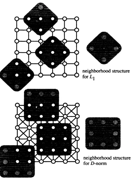
Two graphs together with corresponding homogeneous neighborhood structures are shown
in Figure 2.
The distance $d^{\ell}$
defined by the upper graph $\mathcal{G}$, Manhattan graph, with the neighborhood
structure $\mathcal{H}=\{(-1,0),$ $(0, -1),$ $(0,1),$ $(1,0)\}$ and
$l_{(i,j’)}^{?t}=1$ for all $(i’,j’)\in \mathcal{H}$ (4.2)
is the $L_{1}$ distance on $\mathcal{N}$, while the other
graph, Union Jack graph, with the neighborhood
structure $\mathcal{H}=\{(-1,0), (-1, -1), (0, -1), (1, -1), (1,0), (1,1), (0,1), (-1,1)\}$ and $\ell_{(i,j)}^{\mathcal{H}}=1$ for
all $(i’, j’)\in \mathcal{H}$ defines the $L_{\infty}$ distance. Bertsimas et al. [2] proposed the D-norm for $y\in \mathbb{R}^{n}$
and $\rho\in[1, n]$
as
the optimal value of the linear programmaximize $\sum_{j=1n}u_{j}|y_{j}|n$
subject to $\sum_{j=1}u_{j}\leq\rho$; $0\leq u_{j}\leq 1$ for $j=1,$
neighborhood structure
for$L_{1}$
neighborhood strucmre for D-norm
Figure 2: Graph and neighborhood structure defining a distance on$\mathcal{N}$
The Union Jack graph with
$\ell_{(i’,j’)}^{\mathcal{H}}=\{\begin{array}{l}1 for (i’,j’)\in\{(-1,0), (0, -1), (1,0), (0,1)\}\rho for (i’,j’)\in \{(-- 1, -1), (1, -1), (1,1), (-1,1)\}\end{array}$ (4.3)
defines the D-norm, which gives, by setting the parameter $\rho$ appropriately $(e.g. \rho=\sqrt{2})$, an
in-between of $L_{1}$ and $L_{2}$
.
Suppose the ground distance$d_{(i,j)(k,l)}$ among locations of$\mathcal{N}$ is given as the distance
$d_{(i,j)(k,l)}^{\ell}$
for agraph $\mathcal{G}$ with a homogeneous neighborhood structure. Then for two distinct locations $(i,j)$
and $(k, l)$ there is
an
undirected pathof edges $[(i_{0},j_{0})(i_{1},j_{1})],$ $[(i_{1},j_{1})(i_{2},j_{2})],$$\ldots,$ $[(i_{n-1},j_{n-1})(i_{n},j_{n})]$
such that $(i_{0},j_{0})=(i,j),$ $(i_{n},j_{n})=(k, l)$,
$(i_{r+1},j_{r+1})\in \mathcal{N}_{Q}(i_{r},j_{r})$ for $r=0,$
and
$d_{(i,j)(k,l)}= \sum_{r=0}^{n-1}d_{(i_{r},j_{r})(i_{r+1},j_{r+1})}=\sum_{r=0}^{n-1}p_{(i_{r+1}-i_{r},j_{r+1}-j_{r})}\mathcal{H}$
.
(4.4)Add the constraints
$g_{(i,j)(k_{1}l)}=0$ for all $(i,j)\in \mathcal{N}$ and $(k, l)\not\in \mathcal{N}_{\mathcal{G}}(i,j)$
to problem (R) and denote it by (R), i.e.,
(R)
minimize $dg$
subject to
$(A-B)g=p-q$
$g\geq 0$
$g_{(i,j)(k,l)}=0$ for all $(i,j)\in \mathcal{N}$ and $(k, l)\not\in \mathcal{N}_{\mathcal{G}}(i,j)$,
or
equivalently(R)
minimize $\sum_{(i,j)\in N(k_{\dagger}l)}\sum_{\in \mathcal{N}g(i,j)}\ell_{(k-i,l-j)}^{\mathcal{H}}g_{(i,j)(k,l)}$
subject to $\sum_{(k,l)\in \mathcal{N}_{Q}(i,j)}g_{(i,j)(k,l)}-\sum_{(k,l)\in \mathcal{N}_{G(i,j)}}g_{(k_{2}l)(i,j)}=p_{(i,j)}-q_{(i,j)}$
for all $(i,j)\in \mathcal{N}$
$g_{(i_{2}j)(k,l)}\geq 0$ for all $(i,j)\in \mathcal{N},$ $(k, l)\in \mathcal{N}_{Q}(i,j)$
.
We
see
that problem (R) is equivalent to problem (R).Lemma 4.2. Suppose that the graph$\mathcal{G}$ has the homogeneous neighborhoodstructure $(\mathcal{H}, \ell^{\mathcal{H}})$ and
the ground distance $d_{\underline{(}i,j)(k,l)}$ is given
as
the shortest lengthof
paths in $\mathcal{G}$.
Then every optimalsolution
of
problem $(R)$ is an optimal solutionof
problem $(R)$, and$v(\overline{R})=v(R)$
.
Proof
Let $((i,j)(k, l))$ be an arc of$\mathcal{D}$.
Sincethe ground distance is givenas the shortest length
of paths in $\mathcal{G}$, there is a series of
arcs
$((i_{0},j_{0})(i_{1},j_{1})),$ $((i_{1},j_{1})(i_{2},j_{2})),$
$\ldots,$$((i_{n-1},j_{n-1})(i_{n},j_{n}))$
such that $(i_{0},j_{0})=(i,j),$ $(i_{n},j_{n})=(k, l),$ $(i_{r+1},j_{r+1})\in \mathcal{N}_{\mathcal{G}}(i_{r},j_{r})$ for $r=0,1,$
$\ldots,$$n-1$, and
also the equality (4.4) holds.
Now suppose
we are
givena
feasible flow $g$ ofproblem (R). The above observation impliesthat replacing the
arc
flowof$g_{(i,j)(k,l)}$on arc
$((i, j)(k, l))$ by the path-flow along $((i_{0},j_{0})(i_{1},j_{1}))$,$((i_{1},j_{1})(i_{2},j_{2})),$
$\ldots,$$((i_{n-1},j_{n-1})(i_{n},j_{n}))$ does not change the objective function value.
Repeat-ing this procedure if
necessary,
we will obtain a feasible flow satisfying the additional equalityconstraints
$g_{(i,j)(k,l)}=0$ for all $(i,j)\in \mathcal{N}$ and $(k, l)\not\in \mathcal{N}_{\mathcal{G}}(i, j)$
of (R) without changing the objective function value. This completes the proof. ロ
Theorem 4.3. When the graph $\mathcal{G}$ has the homogeneous neighborhood structure $(\mathcal{H}, \ell^{\mathcal{H}})$ and
problem $(EMD)$ employs the shortest length
of
paths in $\mathcal{G}$as
the ground distance. ThenProof.
Straightforward $hom$ Theorem 3.7 and Lemma 4.2. 口Let $h$ denote the size of$\mathcal{H}$, which is four for the Manhattan graph and eight for the Union
Jack graph. Then comparing (R) with (EMD), the number of variables reducesfrom$m^{2}$ to $mh$.
This will greatly lighten the computational burden.
5
Experimental
Results
We will report
on
someexperimentalresultstodemonstratethe usefulnessofEMDand thecom-putational effectiveness of
our
proposed formulation. The images we used are three sequentialimages of a swimmer in Figure 3 eachof which consists of $32\cross 32$ pixels. By letting weight
$p_{(i,j)}$
(i) (ii) (iii)
Figure 3: Sequential $((iii)arrow(ii)arrow(i))$ swimmer images
be 1 when the grid location $(i,j)$ corresponds to
a
colored pixel and $0$ otherwise, we constructthe three different $32\cross 32$ histograms and compute the dissimilarity among these histograms by
(a) Frobenius
norm
$(i.e., \sqrt{\sum_{i--1}^{m_{1}}\sum_{j--1}^{m_{2}}(p_{(i,j)}-q_{(ij)})^{2}})$,(b) (EMD) with $L_{2}$ ground distance,
(c) (R) with Manhattan graph and (4.2), and
(d) (R) with Union Jack graph and (4.3) with $\rho=1.3$.
All computations
are
conductedon a
personal computer with Core2 CPU $(2.66GHz)$ and $4GB$memory. Problems (b), (c) and (d)
are
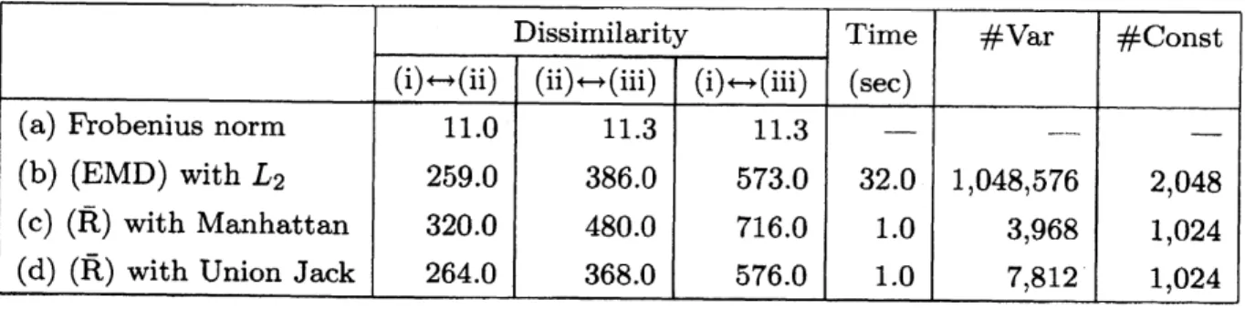
solved by using CPLEX 10.1, OPL Studio 5.1.The column Time of Table 1 shows the average time for computing the three values of
dissimilarity, and the columns $\# Var$ and
#Const
show the number of variables and the numberofconstraints ofeach problem, respectively.
Noteworthypoints
are
in order. Firstly, Frobeniusnorm
(a) provides almost thesame
valueof dissimilarity to all pairs of histograms, while (b), (c) and (d) give relatively large value of
dissimilarity to the pair $(i)rightarrow(iii)$ and successfully reflect the sequential nature of the images.
Secondly, the values of dissimilarity given by (d) are very close to those by (b). This supports
that Manhattan graph with $\rho=1.3$ sufficiently approximates the $L_{2}$ ground distance. Thirdly,
because of the remarkable reduction of problem size (see the columns
#Var
and#Const),
(c)and (d) reduce the computational time sharply in contrast to (b). This reduction would be
especially valuable when applied to image retrieval systems that need to compute dissimilarity
Table 1: Dissimilarity and computational time of Frobeniusnorm, (EMD) and (R)
6
Conclusion
We have proved that the earth mover’s distance problem reduces to a problem with half the
number ofconstraints regardless of the ground distance. Furthermore, we have proposed a
fur-ther reduced formulation when the ground distance comes $hom$ a graph with
a
homogeneousneighborhood structure. The preliminary experiment has shown that the reduction helps
com-pute theearth mover’s
distance
efficiently. In this paper we have assumed that thelocation
hastwo coordinates such
as
$(i,j)$, however, itcan
be generalized toa
higher dimensionalcoordinatesystem with a slight modification.
Acknowledgement
The authors thank Maiko Shigeno, University of Tsukuba for stimulating discussion, and
Jun-ya Gotoh, Chuo University, and Akiko Takeda, Keio University for drawing their attention to
D-norm. This research is supported in part by the Grant-in-Aid for Scientific Research (B)
18310101 of the Ministry of Education, Culture, Sports, Science and Technology of Japan.
References
[1] R.K. Ahuja, T.L. Magnanti and J.B. Orlin, Network Flows. Prentice Hall, 1993.
[2] D. Bertsimas, D. Pachamanova and M. Sim, “Robust Linear optimization under General
Norms,” Operations Research Letters, vol. 32, no. 6, pp. 510-516, 2004.
[3] H. Ling and K. Okada, “An Efficient Earth Mover’s Distance Algorithm for Robust
His-togram Comparison,” IEEE Trans. Pattem Analysis and Machine Intelligence, vol. 29, no.
5, pp. 840-853,
2007.
[4] Y. Rubner, C. Tomasi andL.J. Guibas, “The Earth Mover’s Distance
as a
Metric for ImageRetrieval,” $Int’ l$ J. Computer Vision, vol. 40,
no.
2, pp. 99-121, 2000.[5] Y. Takano and Y. Yamamoto, “Metric-Preserving Reduction of Earth Mover’s Distance
and its Application to Non-negative Matrix Factorization,” Discussion Paper