Distinguishing Discretization and Discrete Dynamics, with Application to Machine Learning, Ecology, and Atomic Physics (Structure and Dynamics of Nonlinear Wave Phenomena)

Distinguishing

Discretization

and Discrete Dynamics, with Application to Machine Learning, Ecology, and Atomic Physics

Karl

Gustafson

*

Abstract. The distinction between the discretizingof acontinuous dynamicalsystem, and

an

anal-ogous

discretedynamical system, is examined. Anumber of critical conceptual misunderstandings

are

identified, in historical context. Implications for the internal structures in machine learning,

ecological dynamics, and atomic

wave

systems,

are

discussed.

51.

Introduction. In arecent paper [GusOO] Ipromised “to analyze from ahistorical perspective how this rather fundamental finding

was

previously missed.” Thefundamental findingreferred to

was

abasicconnection Idiscovered (adozen

years

ago) between widelyusedrecently developed

ma-chine learningalgorithms and the recently developingtheoryof chaotic discrete

dynamical

systems.

My discovery

moreover

implied

some

critical conceptual misunderstandings within both the

ma-chine learning community and the dynamical system community. The first

purpose

ofthe present paper is to keep my promise of [GusOO]. In doing this Iwill go beyond [Gus 00, Gus90, Gus97,

$\mathrm{G}\mathrm{u}\mathrm{s}98\mathrm{a}$, $\mathrm{G}\mathrm{u}\mathrm{s}98\mathrm{b},\mathrm{G}\mathrm{u}\mathrm{s}98\mathrm{c}$, GS99], referring to those

papers

forconvenience. Asecond purpose is to

go beyondmy previous work by discussinghere also certainimplications for the internalstructures

of population dynamics and quantum

wave

system dynamics.

52.

Machine Learning. In

1988 as

aresult of asuccessfulinterdisciplinary proposal for

an

NSF Engineering

Research Center

for Optoelectronic Computing Systemsat the UniversityofColorado

and Colorado State University, Ifound myself responsible for the mathematics and algorithm de-velopment to accompany

an

optical neural network being constructed in hardware. The original

Perceptronmachine learningalgorithm, which was linear, had beenby then superseded by the

im-portant Backpropagation algorithm. Backpropagation

overcame

many learning limitations of the

linear Perceptron. Thiswas accomplished in Backpropagation by introducingnonlinearthresholds,

typically implemented by sigmoids$f(x)=(1+e^{-\beta x})^{-1}$

.

Irefer the reader to the bibliography and

in particular to [RM86] for agood discussion of Badcpropagation (also called other

names

such

as

the $\delta$-rule, multilayer perceptron, etc.). For thepurposesof this paPer,

we

maydescribe

Backprop-’DepartmentofMathematics, UniversityofColorado, Boulder,Colorado 80309-0395,USA

数理解析研究所講究録 1271 巻 2002 年 100-111

agation learning as the building of alearning surface (sometimes _{called the learning landscape)}

in multidimensional space on the basis ofanumber of repetitive training examples (input-0utput pairs).

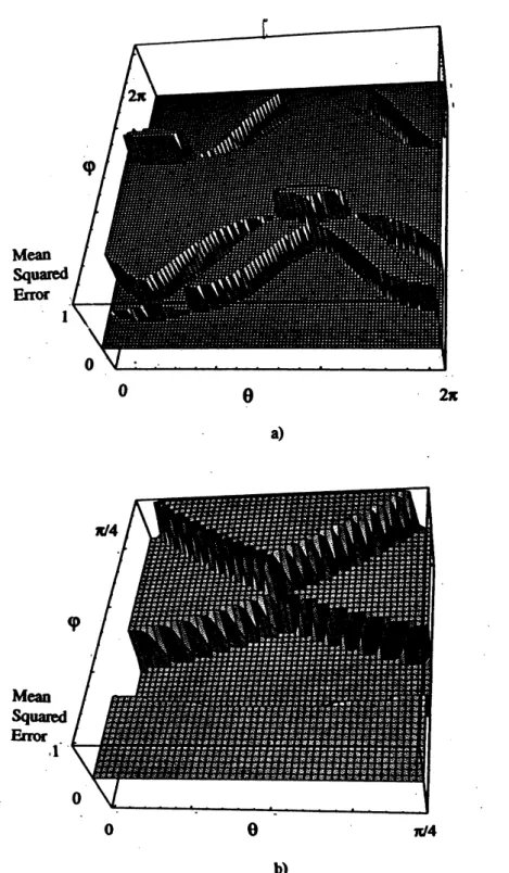
Tofix _{this idea, Ishow in Figure 1such alearning surface from [GG92]. In that (unpublished)} paper,

we

modified Backpropagation to an algorithm we called Anglelearning Backpropagation,

or

Angleprop for short. You may view Figure 1as

depicting

conceptually the

same

type of landscapes the standard Backpropagation algorithm generates

as

aresult of alarge number of training pairs repetitively fed to it. _{Because Backpropagation learns this surface by arepetitive steepest descent}

procedure,

convergence

to the valleys (which carry smaller least squares

error

than mountains

or

plateaus) is often very slow, especially if the previous training iteration put you on

one

of the

plateaus. Our idea in Angleprop

was

to just learn the angles between weights, rather than the weights

themselves.

Iinclude Angleprop here to show you typical Backpropagation

error

surfaces, and because [GG92] was

never

published elsewhere and contains an interesting original idea. See also [WUG94] for

some

recent nice pictures ofsuchlearning surfaces from the Japaneseengineering community.

When we went to implement Backpropagation on the hardware optical neural network, I

learned that theoptical devices

were

not available to usto implement the _{thresholdings. Therefore} wejust took this optical _{data out to adigital computer to do all thresholdingand then went back}

into the optics for the next training epoch. At that point Ilearned that

one

reason

the sigmoid thresholding

was so

popular in the machine learningcommunity

was

that it had the niceproperty that itsderivativeis convenientlyexpressed in termsof itself: $\mathrm{f}’\{\mathrm{x}$)

$=\beta f(x)(1-f(x))$

.

In_particular, in theBackpropagation _{algorithm, this}permits _{the weight changes} $\triangle\omega_{ij}$ tobecalculatedintermsof

currently known network values. AlthoughtheBackpropagationupdate_{formulas becomesomewhat}

complicated_{due to lots ofneural networkinterconnectivityandfeedback,}

_one

_can

_see

that they take the form (at an output node, for simplicity) $\triangle\omega_{ij}=\eta f’(\mathrm{n}\mathrm{e}\mathrm{t})(t_{\ell}-\mathit{0}_{\ell})\mathit{0}_{j}=\eta(t_{\ell}-\mathit{0}\ell)\beta o_{\ell}(1-\mathit{0}_{\ell})\mathit{0}_{j}$

where $t\ell$ is alearning target value,

$\mathit{0}_{\ell}$ is the net output at the current $k\mathrm{t}\mathrm{h}$ iteration,

$\mathit{0}_{j}$ is the

transmitting node value, $\eta$ is apreassigned learning parameter, net is alinear combination of

weighted _{inputs being fed to the nodes, and} $\beta$ is the s0-called gain. If

we

lump

factors

in

we

may

see

that the digitally implemented _{Backpropagation weight updates}

_are

_{each of the form}

$x_{n+1}=\mu x_{n}(1-x_{n})$, which is the discrete _{iterated quadratic map of dynamical}

systems theory

0

₉

$2\pi$ a)

b)

Figure 1: Aplot of theerrorfor theXORproblemversustheangles of the weights

relative to the bias axis andoneoftheweight axes, _{a) Aglobal view of theerror}

surface, _{b)An enlargedviewof solutioninlower lefthandcorner. Noteconstrained}

location of solution

Ilearned in the period 1988-1990that virtually everyone in the machine learning community

was implementing Backpropagation, or similar thresholding multilayer perceptron algorithms, dig-itally. Yet they all

were

also viewing the thresholding

as

it appears in Figure 1, they spoke of it

that way, they viewed it that way, in terms of acontinuous steepest descent minimizing path down

to aleast squares cost function surface. Ihinted at my discovery oflocal discrete quadratic map

dynamics due to digital implementation in [Gus90] but it was only

some

years later after Ihad ascertained to the best ofmy ability that

no one

else shared my discovery, that Ipresented this finding rather completely in $[\mathrm{G}\mathrm{U}\mathrm{S}98\mathrm{c}]$.

Recall that the quadratic mapis well-known to map the interval$0\leqq x\leqq 1$ tozero independent

of initial

guess

$x_{0}$, when $\mu<1$

.

For $1<\mu<3$

one

converges to

anonzero

stationary point. For

$\mu>3$ the quadraticmap may exhibit periodic orbits, aperiodic orbits,

or

chaos. As the simulations

of [$\mathrm{G}\mathrm{u}\mathrm{s}98\mathrm{c}$, GusOO] show, neural networks implementing Backpropagation do exhibit the

same

three qualitative behaviors. Although network connectivity, input and target values; initial weight

choices, learning parameter, etc., all the complexity ofthe learning network architecture and data,

may affect which of these basic behaviors you see, amain point is that this quadraticmap behavior

within aneural network is completely local, i.e., it applies to each individual node in the network.

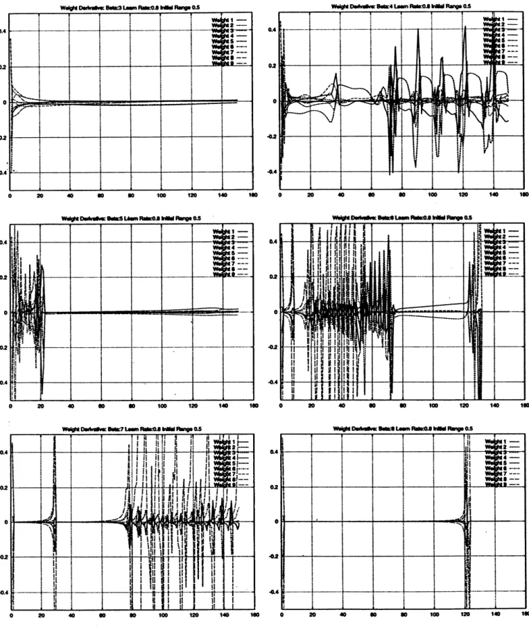
Iillustratethis here in Figure 2. This Figure is the detail of the fourth column of [$\mathrm{G}\mathrm{u}\mathrm{s}98\mathrm{c}$, Figure

2]. As gain $\beta$ increases through values $\beta=3,4,5,6,7,8$, one

sees

weight change behavior varying

from rapid

convergence

to

zero

to intermittent oscillations to oscillatory

nonconvergence.

\S 3.

Historical Comment. Above Ihave pointedouthow the machine learning community missed the fact that

even

the local node-specific learning dynamics

was

that (when implemented digitally)

of the quadratic map of discrete dynamical systems theory. This fact was obscurred by thestrong historical and cultural dogma influenced by the conceptual transition from the linear Perceptron to the nonlinear, smoothly thresholded multilayer perceptron, with its smooth slopes and ravines, upon which you can do gradient descent. That is not to say that others in the machine learning community had not happened onto notions

or

experience of chaos within neural network theory or practice. But (to my knowledge), all

were

confused by failing to distinguish the fundamental differences between continuous and discrete dynamical systems,

or

they

were

influenced too much by analogy,

or

there

was

confusion about onset of chaos being caused by high connectivity

or

large scale. Rather thanrepeatmydiscussions of these things already in [GusOO] and$[\mathrm{G}\mathrm{u}\mathrm{s}98\mathrm{c}]$,let

me

just

Figure 2: Discretequadraticmap irregularitiesin weight changedynamics. Learningparameter$\eta=0.8$

and the initial weights chosen randomly in (-0.5, 0.5), the same initial weights then used for each gain

parameter$\beta$$=3,4,5,6,7,8$. Notethe network internal nonlinear waves, whichoften appeartobe coupled

refer the reader to those papers, with the accompanying summarizingremark here that in [GusOO]

and $[\mathrm{G}\mathrm{u}\mathrm{s}98\mathrm{c}]$ you will find specific reference to, citation to, quotes from, the books of

Devaney, Strogatz, Ott from discrete dynamical systems community, the books of $\mathrm{R}\mathrm{u}\mathrm{m}\mathrm{e}\mathrm{l}\mathrm{h}\mathrm{a}\mathrm{r}\mathrm{t}-\mathrm{M}\mathrm{c}\mathrm{C}\mathrm{l}\mathrm{e}\mathrm{l}\mathrm{l}\mathrm{a}\mathrm{n}\mathrm{d}$ ,

Hertz, Levine, Wiegand-Gershenfeld, Kosko from the machine learning community, all excellent books and outstandingscientists. Ialsocite in [GusOO] and $[\mathrm{G}\mathrm{u}\mathrm{s}98\mathrm{c}]$asignificantnumberofpapers

dealing with chaos in machine learning. Let me add afew more here which have become known to

me and which may be helpful from the historical or conceptual perspectives to anyone who wishes to further pursue this work.

In [SF87]

an

early _{attempt is made to bridge} the recently developed

_{“corinectionist”}

models

(e.g., _{machine learning algorithms and neural network architectures) to actual brain function.}

To quote from the abstract: “Special emphasis is placed in our model on chaotic activity. We hypothesize that chaotic behavior

serves

as

the essential ground state for the neural peceptual

apparatus.” _{However, the point of view of [SF87] is that the role of chaos in the brain is that of}

_a

source ofbackground white noise as observed in EEG studies. Then they adopt the Grassberger-Procaccia et al. model oflow-dimensional deterministic (continuous) dynamical system “strange

attractor” chaos. Also they [SF87, p. 190] “we insist repeatedly that behaviorally relevant neural

information is to be found in the

average

activity of ensembles (as manifested in the EEG) and not in the activity of single neurons.” And [SF87, p. 171] “Connectionist models can certainly be modified to produce _{chaotic and oscillatory behavior, but current theorists have not included}

these behaviors in their models,.

. . .

_{Another [reason] is that engineers have traditionally viewed}

oscillatory and chaotic behavior

as

undesirable and something to be eliminated.” [SF87] also contains an interestingadjoined Open Peer Commentaryby manyof theeminent researchersof the

time, so the whole paper is interesting _{reading. My final point about it is the following. [SF87],} representing the brain-science community, wants to get rid ofthe digital computer metaphor that

the rival _{connectionist community employs. In doing so, [SF87] goes to the continuous dynamical}

system _{chaos models. Thus they have missed my finding that in the digital connectionist models,} single

neuron

chaos

was

already present. The connectionist community missed this fact too.

Another interesting earlierpaper is [Ha83]. The emphasis there is on “higher” neural

process-ing accomplished by incorporating not only current information but also time-delayed connected

information. However there is also

some

discussion_{of individual “trajectories for the netlet,” whic}

in turn leads to discussion ofattractors and the low dimensional (continuous) dynamical system theoryofchaos

so

popular inthe $1980\mathrm{s}$

.

What interests

me

about thisearlypaper is that it actually

presents [Ha83, p. 786] “the parabola $F(x)=4bx(1-x)$, $0<b\leq 1$”as an example of amap which “willbe chaotic forcertain

ranges

of values of$b$and for certain ‘seed’ values of_$x.$” However

again (in my opinion) abetter understanding

was

obscured by not distinguishing and

even more

delineatingthe continuous chaos paradigm ffom the discrete chaos paradigm.

\S 4.

Ecological Dynamics. In [GusOO] Istate: “To May through his influential 1976 paper

[Ma76] belongs much credit for the

resurgence

of recent interest in simple discrete maps, including

the quadraticmap. However, in

our

opinion, the

use

of the words ‘analogous, corresponding’in the transition from population dynamics $P’(t)=aP(t)-bP^{2}(t)$ to

map

equations $y_{n+1}=ay_{n}-by_{n}^{2}$

is misleading. There is

no

way that you

can

discretize the former to obtain the latter in the

sense

of differential equations going to consistent difference equations, e.g.

see

[Gus99]. Succeeding treatises of discrete dynamical systems continue to fall into this (in

our

opinion) trap.77 Iwould like to elaborate this statement here, beyond what Isaid in [GusOO] and $[\mathrm{G}\mathrm{u}\mathrm{s}98\mathrm{c}]$

.

The ordinary differential equation initial value problem $\frac{d}{}dRt=ap-\psi^{2}$,$p(t_{0})=p_{0}$

occurs

widely

in science. In mathematics it falls within the category of Riccati equations. Its solution is easily found to be $p(t)= \frac{ap_{\mathrm{O}}}{b\mathrm{p}\mathrm{o}+(a-b\mathrm{p}\mathrm{o})e^{-a(l-\iota_{0\mathfrak{l}}}}=\frac{1}{1+e^{-\beta l}}$ where in the last equality Itook $a=b=\beta$,

$p_{0}=1/2$, $t=0$

.

Discretization of adifferential equation, e.g., to render adiscrete version of it for numerical solution methods, usually carries the desired requirement of consistency: the true solution, when substituted into the discrete version, has truncation

error

which goes to

zero as

the discretization size becomes arbitrarily small. The obvious finite difference discretization of the initial value

problemis theforward difference $\frac{\mathrm{p}(t+\Delta t)-\mathrm{p}(t)}{\Delta t}=\beta p(t)(1-p(t))$ which is justthedifference quotient

approximation to the first derivative. In this simple instance, consistency just reduces to the fact

that thedifference quotient rule of elementary calculus is aconsistent oneand the sigmoid function

is differentiate.

However,

now

note that discrete quadratic map has virtually

no

connection to the continuous

parameter _{differential equation from the point of view of discretizing the former to get the latter.}

Nor can you work back ffom the latter,

as

if it

were

adiscretization, to get theformer. Ifyou try

a

few obvious discretization schemes, you will

see no

naturalconnections between the two equations.

Therefore Ithink agood word is incommensurate: the population dynamics equation and the

quadratic map equation, although analogous, are incommensurate.

\S 5.

Historical Comment. May [Ma76] popularized the mathematics of iterated maps and imagined _{them to be apossible explanation of the oscillations he had observed in population}

dynamics. Gleick [G187] gives _{agood account of this story. Then [G187, p. 80]: “May realized}

that the astonishing structures he had barely begun to explore had no intrinsic connection to biology.” But [G187] does not develop this latter statement. Let

me

do

so

here. If you look at [Ma81] you will find alowered emphasis

on

the potential

use

of iterated

maps

for such ecological population modelling. May clearly [Ma81, Chapter 2] now restricts the conceptual use of

one-dimensional quadratic maps to models for single populations. The assumption has to be [Ma81, p. 6] that “generations

are

nonoverlapping and growth is adiscrete process (first order difference

equations).” Then for continuous growth, differential equations

are

proposed [Ma81, section 2.2].

However, to fit population data, time delays

are

also allowed into these equations. This is okay, these continuous population models have served ecological dynamics well, but it should be noted at this point that mathematicians’ know well that differential-delay equations can model awide

variety of dynamics. When we get to the main section 2.3 of [Ma81], Discrete growth (difference

equations),

some

actual ecological examples

are

claimed. However, the discussion quickly slides away from the biology and into the iterated map _{mathematical lore. Without asingle specific} ecological data set yet, we

come

to the statement [Ma81, p. 17]: “To see mathematical ecology informing theoretical physics is apleasing inversion of the usual order of things.” Without any ecology yet, this would appear to

me

to be inverted logic. When

we

do get to population data,

one

resorts to time delay

or

thecontinuous dynamics models. In Fig. 2.6 [Ma81, p. 21], Fig. 6[Ma76],

we find only

one

data point in the “chaos” region, and that not for aquadratic _{equation, rather}

for afit by $y_{t+1}\cong 60\mathrm{y}\mathrm{t}(1+y_{t})^{-10}$.

To this day, confusion persists about the appropriate roles ofdiscrete and continuous chaos. By this Imean, respectively: chaoticiterative dynamicsproducedby

an

iterateddiscretedynamical system, and chaotic dynamics produced _{by the continuous time evolution of anonlinear system of}

ordinary differentialequations. For example, beyond the popular quadratic map, another popular

discretedynamical system is thequadraticHenon-Heilesmap,

see

[Ta89]. Perhaps the mostpopular

exampleof_{acontinuous chaoticdynamical systemisthefamousquadraticLorenzsystemwhich}

_was

an

extreme simplification

of

the partial

differential

equations

of

meteorology.

See

the discussions in [G187], [Ta89], and elsewhere. Both the Lorenz continuous dynamical system and the Henon

discrete dynamical systempossess strange attractors. What Iam asserting above in Section 4and

throughout this paper is that the algebraic similarities in $fom$ between the discrete dynamical

systems and the continuous dynamical systems equations

can

be critically misleading, and

one

cannot assert apriori any ‘corresponding’ behavior in their dynamics without afurther analysis

which would (unlikely in most instances) prove such.

How this confusion happens? Iwould like to identify two key factors, although there

are

certainly others. Let

me

briefly present these two factors: analogy and vocabulary. The point I would like to make here is that Analogy although apowerful mental function, should be regarded as asubjective reasoning. Always it should then be placed into an objective analysis. Subjective reasoningrelies

on

experience-based intuition and

can

be very powerful but

can

also lead to serious

errors

unless checked by deductive systematic testing. Right brain and leftbrain cannot trusteach

other and theircoexistence may beviewed as avaluable systemof checksandbalances. Thesecond

factor Iwish to identify is vocabulary. For example,

one

finds the term logistic used in the literature for both the continuous population equation and discrete quadratic map. Also the

same

function is called both the logistic function and the sigmoid function. Such vocabulary failures of precision

can translate into conceptual confusions.

56.

Atomic Physics. Next Iwould like to turn to athird field ofscientific endeavor, Atomic Physics, where Ibelieve caution should be exercised to avoid critical misunderstandings due to insufficient

care

in distinguishingcontinuous and discrete dynamical systems. Ihaven’t discussed

thissituation previously. Theproblems arise in attempts to model quantum dynamics by classical

Hamiltonians

so

that

one can

actually calculate approximate bound states and their energies

as

periodic orbitals

as

if they

were

in the old Bohr “solar system” quantum mechanics. Within

the mathematics of quantum mechanics these theories and techniques go under the names

Born-Oppenheimer approximation, WKB method, Bohr-Sommerfeld quantization. In our conference volume [GR81] youwillfind several articles

on

thistopic. Ialso recommend theconferencevolume [Hi83] for asimilar perspective. Also

see

[Ta89], to which Iwill refer below. Iwill also refer to [BR97], with all due respect and apologies to my colleague William P. Reinhardt with whom Iput out the book [GR81] about twenty years ago

Without getting into the details, given aquantum mechanical Hamiltonian $H$ viewed

semi-classically, the density of states per unit energy $\rho(E)$ is given by _{$\rho(E)=Tr[\delta(E-H)]=\sum_{n}\delta(E-$}

$E_{n})$ where C5 is the delta function and the $E_{n}$

are

the distinct eigenvalues of the Hamilton-ian. By Fourier Transform $\delta(E-H)=\frac{1}{2\pi\hslash}\int_{-\infty}^{\infty}e^{iEt/\hslash}e^{-iHt/\hslash}dt$, the density becomes _$\rho(E)=$ $\int_{-\infty}^{\infty}e^{iEt/\hslash}Tr(e^{-iHt/\hslash})dt=\frac{1}{2\pi\hslash}\int_{-\infty}^{\infty}e^{iHt/\hslash}\int\langle q, e^{-iHt/\hslash}q\rangle dqdt$ where the last integral represents

integrationof the expectation values

over

all configuration states $q$ at time $t$ in the evolution. The

semiclassical approximation then is achieved by approximating this expectation value integrand by $\langle q_{1}, e^{-iHt/\hslash}q_{2}\rangle\sim e^{i\phi(q_{1\prime}q_{2})/\hslash}$ where $\phi(q_{1}, q_{2})$ is the action integral along the classical trajectory connecting $q_{1}$ and $q_{2}$ in time interval $[0, t]$. In other words, the quantum

averagirig

is replaced by

asingle frequency oscillation. This leads via the

now

classical Hamiltonian dynamics to arequire-ment that the values of$q$ which actually contribute in this stationary phase

sense

to the integral

must lie

on

aperiodic trajectory. See [BR97] and [Ta89] for more details.

It is well-known that classical Hamiltonian systems may exhibit chaos. For example [Ta89] the Henon-Heiles Hamiltonian $H= \frac{1}{2}(p_{x}^{2}+p_{y}^{2}+x^{2}+y^{2})+x^{2}y-\frac{1}{3}y^{3}$ exhibits chaotic Poincare

cross

sections. There

are

many other examples and it can be said that the thrust of quantum

chaos studies are motivated by these classical Hamiltonian chaotic dynamical systems. [BR97, $\mathrm{p}$. 83] are careful to point out that true quantum systems do not typically display chaos in the

sense

ofexponential sensitivity to initial state. They

are

careful to distinguish (I) quantized chaos, (II)

semi-quantum chaos, (III) quantum chaos. It is really (I) whichdominates most current modelling.

Thus

one

mayconsidernotonly periodicorbits from the stationaryphase approximationIdescribed

above, but also aperiodicorbits and

more

irregular orbits in thesame setting. [Ta89, p. 229] is also very careful to point out that the steps in the semiclassical approximation from the Schr\"odinger

partial differential equation to aclassical Hamilton-Jacobi equation, “is very subtle.” As Planck’s

constant Ais taken to zero, one is neglecting the $i\hslash\nabla^{2}S/2m$ term in the limit. Moreover $\hslasharrow 0$

corresponds to “ever

more

rapid oscillations in the

wave

function.” Here $S=S(q, t)$ represents

a

single phase evolution in the

wave

function $\psi(q, t)=e^{iS/\hslash}$ resultingfrom aseparation of variables.

They go

on

to make clear that “It is completely wrong to think that

someone can

somehow write

quantum mechanical quantities as classical quantities plus an expansion of corrections in power of

$\hslash$

.

”

\S 7.

Historical Comment. My

concern

about the models presented above inSection 6is the mix

of discrete and continuous dynamical systems employed in this current research in atomic physics. This mix is found throughout [BR97] and [Ta89] and elsewhere. It is too easy to imagine that the

discrete model’swave systemdynamics somehowreally depict what is happening in the continuous

model’s

wave

system,

even

when staying completely within the frame of classical Hamiltonian systems. Although [BR97] and [Ta89]

are

careful to put in qualifying provisos, there still is the inference that

one

really is modelling quantumchaos, i.e. stated

more

carefully, quantum evolutions which depend on an underlying chaos. The fact that underlying discrete nonlinear chaotic phase-space dynamics

can

be treated in terms ofstate space (e.g., probability distributions) functions

over

the phase space is demonstrably true in statistical mechanics,

see e.g.

[Gus97]

or

[GR81] and citations therein. But it onlyholdstrue in that situation for rather special ’Kolmogorov’ dynamical systems and

on

compact phasespaces. Thus the “manifestations of chaos in atomic and molecular physics” [BR97] must be taken

as

experimentally

or

conceptually inspired rather than theoretically proven. Finally, is there really any need for such chaos models in atomic physics? The physical evidence presented in [BR97] and [Ta89] is

meager

at best. And amanifestation ofchaos is not proofof true underlying physical chaos.

58.

Conclusions. The three ‘stories’ Ihave given here illustrate the force of fashion within the scientific enterprise. The machine learning community followed afashion ofsmooth learning surfaces and did not

see

and did not want the chaos which Iidentified

as

inadvertently introduced through digital, i.e., discrete, implementation of nonlinear thresholdings. The ecological dynamics community became entranced with afashion of chaos

even

though chaos

was

not in their population dynamics. The atomic physics community created afashion of quantum chaos which n0-0ne has

yet

seen.

References

[BR97] Bliimel, R. and Reinhardt, W. P., Chaos in AtomicPhysics, Cambridge University Press,

Cambridge, 1997.

[G187] Gleick, J., Chaos: Making a Neeu Science, Viking, New York, 1987.

[GusOO] Gustafson, K., Chaos in discrete learningsystems, Chaos, Solitons and Fractals 11 (2000),

321-327

[Gus90] –, Reversibility in neural processing systems, in: Statistical Mechanics

of

Neural Networks, (L. Garido, ed.), Lecture Notes in Physics 368, Springer, Berlin, 1990,

269-285.

[Gus97] –, Lectures on Computational Fluid Dynamics, Mathematical Physics, and

Linear Algebra, World Scientific, Singapore, 1997.

[Gus98a] –. Internal dynamics of Backpropagation learning, in: Proc. Ninth Aus-tralian

_Conference

on Neural Networks, (T. Downs, M. Prean, M. Gallagher, eds.), Uni-versity of Queensland, Brisbane, 1998, 179-182.

[Gus98b] –, Ergodic learning algorithms, in: Unconventional Models

of

Computa-tion, (C. Calude, J. Casti, M. Dinneen, eds.), Springer, Singapore, 1998, 228-242.

[Gus98c] –, Internal sigmoid dynamics in feedforward neural networks,

Connection

Science 10

(1998),

43-73.

[Gus99], –, Partial

Differential

Equations and Hilbert Space Methods, Dover

Pub-lications, New York, 1999.

[GG92] , Gustafson, K. and Goggin, S., Anglelearning Backpropagation, (1992, unpublished).

[GR81] Gustafson, K. and Reinhardt, W. P., Quantum Mechanics in Mathematics, Chemistry, and Physics, PlenumPress, NewYork, 1981.

[GS99] Gustafson, K. and Sartoris, G., Assigning initial weights in feedforard neural networks, in: Proc. 8th IFAC Symposium on Large Scale Systems, (N. Koussoulas, P. Groumpos,

eds.), _{Patras, Greece, July 1998, Pergamon Press, N.Y. 1999, 1108-1113.}

[Ha83] Harth, E., Orderand chaos in neural systems: anapproachto the dynamics of higher brain functions, IEEE Trans, on Systems, Man, and Cybernetics, $\mathrm{S}\mathrm{e}\mathrm{p}\mathrm{t}./\mathrm{O}\mathrm{c}\mathrm{t}$. 1983, 782-789.

[Hi83] Hinze, J. (ed.), _{Energy Storage and Redistribution in Molecules, Plenum Press, New York,}

1983.

[Ma76] May, R., Simplemathematicalmodelswithverycomplicateddynamics, Nature261 (1976), 459-467.

[Ma81] –(ed.), Theoretical _{Ecology: Principles and Applications, 2nd Ed.,} Black-wellScientific Publications, Oxford, 1981.

[RM86] Rumelhart, D. and McClelland, J. et al, Parallel Distributed Processing, Vols. I, II, MIT Press, Cambridge, MA, 1986.

[SF87] Skarda, C. and Freeman, W., How brains make chaos in order to make

sense

of the world,

Behavioral and Brain Science 10 (1987), 161-195.

[Ta89] Tabor, _{M., Chaos and Integrability in Nonlinear Dynamics, Wiley, New York, 1989.}

[WUG94] Watanabe, T., Uchikawa. Y., and Gouhara, K., Experimental studies ofmemorysurfaces

and learning surfaces in recurrent neural networks, Systems and Computers in Japan 25,

No. 8 (1994), 27-39, (Denshi Joho Gakkai Ronbunshi J76-D-II, No. 5, 1993,

_1055-1065