Some inverse problems and fractional calculus (New Developments of Functional Equations in Mathematical Analysis)

Some

inverse

problems

and

fractional

calculus

Yutaka Kamimura *

Department of Ocean Sciences, Tokyo University ofMarine Science and Technology,

4-5-7 Konan, Minato-ku, Tokyo 108-8477, email: [email protected]

Several inverseproblemsinphysics

are

modeled intermsofnonlinearintegralequations

ofthe Abel type. The main aim of this survey article isto show amethod withfractional

calculus iscommonly effective for proving the global existence ofsolutions to the integral

equations.

A typical inverse problem reduced to

a

nonlinear integral equation of the Abel type

is the problem to determine

a

restoring force of the Newtonian equation such that the

equation hasaprescribedhalf-period as afunction of thehalf-amplitudeof of the solution:

Problem 1 Determine a nonlinearity $g$ of

an

equation $=d^{2}udt+g(u)=0$

so

that, for each

$x\in(0, r]$, a solution $u(t)$ of the equation with the stationary (maximal) value $x$ has a

half-period $T(x)$ that is

a

prescribed function of$x$

.

Figure 1: Problem 1.

As is easily verified by a standard discussion (see, e.g., [16]), Problem 1 is reduced to

the integral equation:

$\sqrt{2}\int_{0}^{x}\frac{dy}{\sqrt{\int_{y}^{x}g(u)du}}=T(x)$, $0\leq x\leq r$

.

(1)

Here $r>0,$ $T(x)$ is a prescribed, positive function, and we seek a solution $g$ that is

continuous on the interval $[0, r]$, positive on the interval $(0, r]$. The uniqueness of

a

continuous solution$g$of(1)

was

establishedby Opial [10]. The existence resultfor Problem

1 was firstly obtained by Urabe [15, 16], which showed that (1) admits a solution $g$ if $r$

is small, under the assumption that $T$ has a Lipschitz continuous derivative. This local

existence result

was

improved by Alfawicka [1], which showed that (1) admits a solution

$g$ if $r$ is small, under the assumption that $T$ itself is Lipschitz continuous. However

whether the solution exists globally (in the

sense

that $r$ is arbitrary) had been

a

well-known open problem in the field ofinverse problems, until the author [9] has closed this

open problem recently by proving the following global versionofthelocalexistence result

due to Alfawicka.

Theorem 2 ([9]) Given a Lipschitz continuous, positive

_function

$T$

on

the interval $[0,r]$,

there exists

a

(unique) solution $g$

of

(1) that is continuous

on

$[0, r]$ andpositive

on

$(0,r]$

.

We give

an

example indicating the meaning ofTheorem 2:

Example 3 Let $-$

oo

$<\alpha<1$, let $G(x)$ be the inverse function of the incomplete beta

function

$x(t):= \int_{0^{s^{-f}(1-s)^{-\alpha}ds}}^{t_{1}}$,

and let $T(x)$ be afunction defined by

$T(x)=\sqrt{2}\pi F(\alpha,$$\frac{1}{2},1;G(x))$

with the Gauss hypergeometric function $F(\alpha, \beta, \gamma;t)$

.

Then the solution _$g$ of (1) is given

by

$g(x)=G(x)^{\pi}1(1-G(x))^{\alpha}$ , $0\leq x<x_{0}$ $:=B( \frac{1}{2},1-\alpha)$

.

One

can

verify (see [9]) that $g$ satisfies (2) with the function $T(x)$ for $0\leq x<x_{0}$

.

Figure 2: $g(x)$ and$T(x)$ for $\alpha\in(0,1)$

In the

case

$-\leq\alpha<1$ (see the upper part in Fig 2), the prescribed function $T(x)$ is

increasing monotonically from $\sqrt{2}\pi(=T(O))$ to $+\infty$

as

$x$

moves

from$0$to $x_{0}$. Then

Theorem 2 when

we

take $r$ in $(0, x_{0})$

.

The lower bound$\alpha=\frac{1}{2}$ inthis

case

is corresponding

to the simple pendulumsince$g(x)= \frac{1}{2}\sin x$ and$T(x)= \sqrt{2}\pi F(\frac{1}{2},$$\frac{1}{2},1;s^{2}\frac{x}{2})$ for $\alpha=\frac{1}{2}$

.

In the

case

$0< \alpha<\frac{1}{2}$ (see the lower part in Fig 2), the prescribed function _$T(x)$ is

increasing monotonically from $\sqrt{2}\pi(=T(0))$ to $T(x_{0})=\sqrt{2\pi}\Gamma(1/2-\alpha)/\Gamma(1-\alpha)$

as

$x$

moves

from $0$ to _{$x_{0}$}. However, in this case, _$T(x)$ is not Lipschitz continuous at

$x_{0}$

.

Hence,

as

well

as

in the

case

$-\leq\alpha<1$, Theorem 2 is applicable by taking $r$ in $(0, x_{0})$

.

Notice

that we

are

not able to take $r$

as

$x_{0}$ because $g(x)=0$ at _{$x=x_{0}$}

.

The lower bound $\alpha=0$

in this

case

is corresponding to

a

spring with

a

homogeneous elasticity, since $g(x)= \frac{1}{2}x$

and $T(x)\equiv\sqrt{2}\pi$ for $\alpha=0$. In the

case

$0\alpha<0$the prescribedfunction _$T(x)$ is decreasing

monotonically from $\sqrt{2}\pi(=T(0))$ to $T(x_{0})=\sqrt{2\pi}\Gamma(1/2-\alpha)/\Gamma(1-\alpha)$

as

_$x$

moves

from

$0$ to _{$x_{0}$}. However, either in this case, _$T(x)$ is not Lipschitz continuousat

$x_{0};g(x)$ is going

to $+\infty$

as

_{$xarrow x_{0}$}

.

Theorem 2 is also applicable by taking

$r$ in $(0, x_{0})$

.

The proof of Theorem 2 is crafted by an appropriate combination of of fractional

calculus and successive approximations in [9]. Here we explain only a core of it. By

letting $x(t)$ be the inverse function of$t= \int_{0}^{x}g(u)du$, equation (1) is rewritten

as

$\frac{\sqrt{2}}{2\pi}\int_{0}^{t}\frac{T(x(s))}{\sqrt{t-s}}ds=x(t)$

.

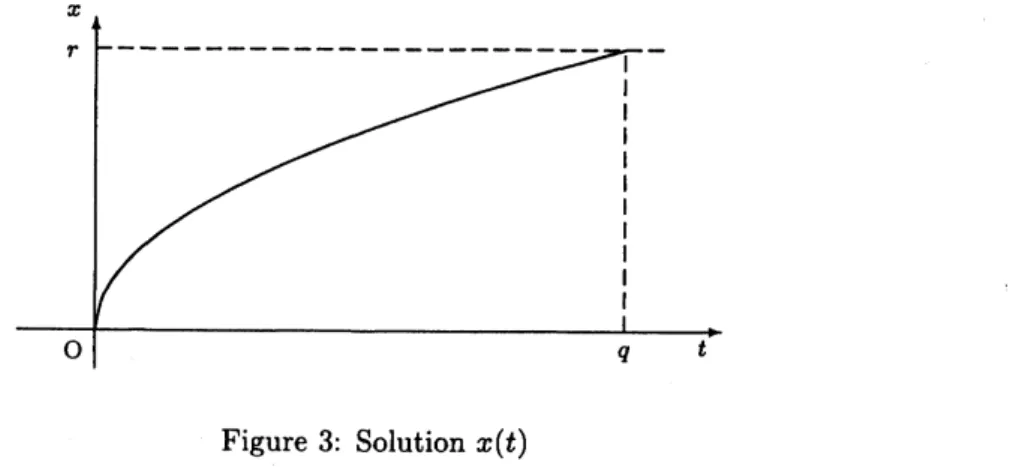
(2)

Applying a method of successiveapproximationswe

can

get

a

solution$x(t)$ of thisequation

reaching $r$ (see Figure 3). So our task is to show that _$x(t)$ is monotonically increasing,

because $g$ is the derivative of the inverse function of $x(t)$.

Figure3: Solution $x(t)$

Proposition 4 Let$T$ be a Lipschitz continuous

function

on an interval containing$0$ and

assume

that $T(O)>0$.

_If

a continuous

_function

$x(t)$

defined

on

some

bounded, closed

interval $[0, q]$

satisfies

(2) then$x(t)$ is

differentiable

and the derivative _$x’(t)$ is _positive

on

$(0, q]$

.

The proof of this proposition is based upon the fractional calculus associated with a

Riemann-Liouville integral operator $I^{\delta}$ defined by

($\Gamma$ is the Gamma function) and and a corresponding differential operator $D^{\delta}$ defined by

$D^{\delta}=DI^{1-\delta}$, where $D$ is

a

standard differential operator $D=d/dt$

.

Generally speaking,

the $Remam-Li_{ouV}m_{e}$ integral operators improve the H\"older continuity of

functions

by

their order $\delta$, while the $Riemam-Li_{ouV}m_{e}$ differential operators $D^{\delta}$ have the

converse

character (see Samko, Kilbas and Marichev [12]). We

use

this mapping property of the

Riemann-Liouvilleoperatorswithin theframework of

a

H\"olderspace, whichis

a a

modified

version of the result dueto Hardy and Littlewood [2].

First

we

note that equation (2) is written

as

$I^{1} z\frac{Tox}{\sqrt{2\pi}}=x$.

Applying the operator $D^{1}\pi$

to this equality

we

get

$\frac{Tox}{\sqrt{2\pi}}=I^{1}zx’$,

and, in tum, letting $\epsilon$ be asmall, positive number and applying the operator

$D^{1}z$

to this

resulting equation, we arrive at

$D^{1-\epsilon} \frac{Tox}{\sqrt{2\pi}}=D^{\frac{1}{2}-\epsilon}x’$

.

If the set $\{t\in(0, q]|x’(t)=0\}$

were

not empty thenwe

can

show that $(D^{1}\Sigma^{-\prime})(a)\leq-\rho<0$

at the smaUest point in the set, where $\rho$ is a positive number independent of$\epsilon$. On the

otherhand we

can

get

$\lim_{\epsilonarrow 0}(D^{1-\epsilon}\frac{Tox}{\sqrt{2\pi}})(a)=0$

The assumption that $T$ is Lipschitz continuous is used essentially at this stage. In this

waywehavegotacontradiction. Thisisan outlineof the proofofProposition Proposition

4. We wish to point out that this proposition is of independent interest in the field of

integral equations, apart ffom Problem 1.

Problem 1 is interpreted

as a

part of

an

inverse bifurcationproblem (for several inverse

bifurcation problems,

see

Iwasaki and Kamimura [3, 4], Kamimura [7], Shibata [13]$)$. As

is well-known in ageneral bifurcation (see, e.g., Rabinowitz [11]), if $f$ is continuous with

$f(0)>0$ then the first bifurcating branch of the nonlinear eigenvalue problem

$\{\begin{array}{l}u’’+\lambda uf(u)=0 on (0,1),u(0)=u(1)=0,u\neq 0 on (0,1).\end{array}$ (3)

bifurcates at the point $( \frac{\pi^{2}}{f(0)},$$0)$ from the trivial solution. By the condition that $u\neq 0$ on

the interval $(0,1)$, each solution $u$ of (4) is positive or negative in the interval. Hence the

solution has its maximum value or minimum value at the middle point $\frac{1}{2}$ in the interval

(see Figure 4). By

means

of the value $h$,

as a

projection into $(0, \infty)\cross I$ of the first

Figure 4: Solution of equation (3).

$\Gamma(f)$ _$:=$

{

$(\lambda,$$h)\in(0,$ $\infty)\cross I|$ョ$u\in C^{2}[0,1]$ satisfying (3) and $u( \frac{1}{2})=h$

},

(4)

where $I$ is a bounded, closed interval containing $0$. Let us confine ourselves in the case

where $f(u)>0$ on $I$ in what follows. It is easy _$0$ see that the set _$\Gamma(f)$ is represented

as

$\Gamma(f)=\{(\lambda(h), h) : h\in I\backslash \{0\}\}$ via apositive function $\lambda(h)$ defined by

$\lambda(h)=2(\int_{0}^{1}\frac{dt}{\sqrt{\int_{t}^{1}sf(hs)ds}}I^{2}$ (5)

In this way we may define a correspondence

$\mathcal{B}:f(u)\mapsto\lambda(h)$,

which

we

refer to

as

the bifurcationtransform. It should be noted that the trivial function

$f\equiv f(O)$ is mapped by the bifurcation transform $\mathcal{B}$ to the trivial bifurcation

$\lambda(h)\equiv\frac{\pi^{2}}{f(0)}$,

which is corresponding to the linear case.

Figure 5: Bifurcation Transform.

Our inverse bifurcation problem is to ask whether $f$

can

be recovered from $\lambda(h)$, which

Problem

5

1. (Existence)

Given a

positive function $\lambda$

on

$I$, does there exist

a

positive function $f$

on

$I$ such that $Bf=\lambda$ ?

2. (Uniqueness) Is $f$ unique for each $\lambda$ ?

3. (Stability) Does $f$ depend

on

$\lambda$ continuously ?

4. (Reconstruction) Can

one reconstruct

$f$ from $\lambda$ ?

An

answer

to questions 1 and 2 of Problem 5 is obtained

as an

immediate rewriting of

Theorem 2:

Theorem 6 Given

a

Lipschitz continuous, positive

_function

$\lambda$

on

_$I$, there exists

a

unique

continuous

_function

$f$

on

I such that$\mathcal{B}f=\lambda$

. The

function

$f$ is obtainedin

a constructive

way.

Notice that Theorem6 is aglobalresult in the fieldofinversebifurcation problems. In

addition, since

a

method ofproofto Theorem 2 is constructive (recall that thesolution of

$x=x(t)$ to equation (2) is obtained bysuccessive approximations),

we

can

get

a

general

strategy for question 4, namely, for reconstruction of the nonlinearity $f$

.

When

one

considers the bifurcation transform $\mathcal{B}$

as a

map, the space of Lipschitz continuous functions is not

so

suitable, because the inverse image of the space via the transform is not well-characterized. So, instead of the space of Lipschitz continuous

functions,

we

introduce the following H\"older-like spaces with $\alpha\in(0,1]$:

$C^{0,\alpha}(I)_{1};= \{\phi\in C(I):||\phi||_{0,\alpha,1}:=\sup_{h\in I\backslash \{0\}}\frac{|\phi(h)|}{|h|}$

$+ \sup_{h,k\in I\backslash \{0\},h\neq k}\frac{||h|^{\alpha-1}\phi(h)-|k|^{\alpha-1}\phi(k)|}{|h-k|^{\alpha}}<\infty\}$ ,

$C^{1,\alpha}(I)_{1}:=\{\psi\in C(I)\cap C^{1}(I\backslash \{0\}):\psi(0)=0,$ $h\psi^{f}(h)\in C^{0,\alpha}(I)_{1}\}$

.

Equipped with the

norms

$||\phi||$ $:=||\phi||_{0,\alpha,1}$ and $||\psi||;=||h\psi’(h)||_{0,\alpha,1}$ respectively, the

spaces$C^{0,\alpha}(I)_{1}$ and $C^{1,\alpha}(I)_{1}$

are

Banach spaces. A suitable choice ofmetric spacessetting

for the transform $\mathcal{B}$ is the combination of

$\mathcal{M}^{0,\alpha}(I)_{1}:=\{f\in C_{+}(I):f(h)-f(0)\in C^{0,\alpha}(I)_{1}\}$

and

$\mathcal{M}^{1,\alpha-z}(I)_{1}:=1\{\lambda\in C_{+}(I):\lambda(h)-\lambda(0)\in C^{1,\alpha-\frac{1}{2}}(I)_{1}\}$ ,

with $\alpha\in(\frac{1}{2},1)$, where $C_{+}(I)$ denotes the set of continuous, positive functions and the

metrics of $\mathcal{M}^{0,\alpha}(I)_{1}$ and $\mathcal{M}^{1,\alpha-\frac{1}{2}}(I)_{1}$ are defined by

$d(f_{1}, f_{2}):=|f_{1}(0)-f_{2}(0)|+||(f_{1}(h)-f_{1}(0))-(f_{2}(h)-f_{2}(0))||_{0,\alpha,1}$

and

$d(\lambda_{1}, \lambda_{2}):=|\lambda_{1}(0)-\lambda_{2}(0)|+||(\lambda_{1}(h)-\lambda_{1}(0))-(\lambda_{2}(h)-\lambda_{2}(0))||_{1,\alpha-\frac{1}{2},1}$

respectively. With the aid of these metric spaces, we have

an answer

to questions 1-3 of

Theorem 7 Let $\frac{1}{2}<\alpha<1$

.

Then $\mathcal{B}$ is

a

homeomorphism

of

$\mathcal{M}^{0,\alpha}(I)_{1}$ onto $\mathcal{M}^{1,\alpha-}\pi(I)_{1}1$

.

Theorem 7implies that, for each first bifurcating branch $\lambda\in \mathcal{M}^{1,\alpha-\frac{1}{2}}(I)_{1}$, there exists

a

unique nonlinearity $f$ in $\mathcal{M}^{0,\alpha}(I)_{1}$ realizing the first bifurcating branch (the

answer

to

question 1-2), and in addition, that the correspondence $\lambda\mapsto f$ is continuous with respect

to the topology of $\mathcal{M}^{0,\alpha}(I)_{1}$ and $\mathcal{M}^{1,\alpha-\frac{1}{2}}(I)_{1}$ induced from the

metrics of these spaces

(the

answer

to quention 3), providedthat $\alpha\in(\frac{1}{2},1)$

.

Since the space$\mathcal{M}^{0,1}(I)_{1}$ is

no

other

than that ofLipschitz _{continuous functions, Theorem 6 can be regarded}

_as

_{the limit}

_case

of Theorem 7

as

$\alphaarrow\frac{1}{2}+0$, though the conclusion in Theorem 7

seems

to break down

when $\alpha=\frac{1}{2}$

.

We omit the proof _{of Theorem 7, which is rather long and technical, deviating from} the aim of this article.

In this article we have discussed a method with fractional calculus that is applicable

in proving the global existence of solutions to integral equations related with inverse

problems. The method is also available for

a

heat conductivity determinationproblem:

Problem 8 Given

_functions

$f(t),g(t)$, _detemine $a(t)$ so that the pambolic system

$\{\begin{array}{l}u_{t}=a(t)u_{xx},u(x, 0)=0,u(0, t)=f(t),-a(t)u_{x}(0, t)=g(t),\end{array}$

admits a bounded, solution $u(x, t)$.

$0<x<\infty,$

$0<t<T$

;

$0\leq x<\infty$;

(6)

$0\leq t<T$;

$0<t<T$

This inverse problem was studied by Jones [5, 6], Suzuki [14], Kamimura [8]. The

original idea offractional calculus applicable _{to inverse} problems can be found in [8],

References

[1] B. Alfawicka, Inverseproblems connected with periods _ofoscillations describedby$\ddot{x}+g(x)=0$, Ann.

Polon. Math. 44 (1984), 297-308.

[2] G.H. Hardy and J.E. Littlewood, Some properties _{of fractional} integrals. I, Math. Zeitschrift, 27

(1928), 564-606.

[3] K. Iwasaki and Y. Kamimura, An inverse _bifurcationproblem and an integral equation _of the Abel

type,Inverse Problems 13 (1997), 1015-1031.

[4] K. Iwasaki and Y. Kamimura, Inverse _bifurcation problem, singular Wiener-Hopf equations, and

mathematicalmodels in ecology, J. Math. Biol. 43 (2001), 101-143.

[5] B. F. Jones Jr. , The detemination _of a _coefficient in a parabolic _differential equation, Part I,

existence and uniqueness, J. Math. Mech. 11 (1962), 907-918

[6] B. F. Jones Jr. , Various methods_forfinding unknown _coefficients in parabolic_differential equations,

Comm. Pure. Appl. Math. 16 (1963), 33-44.

[8] Y. Kamimura, Conductivity

_{identification}

inthe heat equation by the heat flux,J.Math. Anal. Appl.

235 (1999), 192-216.

[9] Y. Kamimura, Global $e\dot{m}$tence ofa restoring

force

realizing aprescrived half-period, J. Differential

Equations, in press.

[10] Z. Opial, Surles peiiodes des solutions de l’\’equation

_{differentielle}

$x”+g(x)=0$. Ann. Polon. Math.

10 (1961), 49-72.

[11] P.H.Rabinowitz,NonlinearSturm-Liouvilleproblem_forsecond order ordinary_differentialequations,

Comm. Pure Appl. Math. 23 (1970), 939-961.

[12] S.G. Samko, A.A. Kilbas, O.I. Marichev, Fractional integrals and derivatives, Gordon and Breach,

Switzerland, 1993.

[13] T. Shibata,$L^{q}$-inverse spectral problems

for

semilinearSturm-Liouvilleproblems, Nonlinear Analysis

69 (2008), 3601-3609.

[14] T. Suzuki, MathematicalTheory of Applied Inverse Problems: Sophia Kokyuroku in Math. Vol. 33,

Sophia University, Tokyo, 1991.

[15] M. Urabe, The potentid

_force

yielding a periodic motion whose period is an arbitrary continuous

function

ofthe amplitude _ofthe velocity, Arch. Rational Mech. Anal. 11 (1962), 27-33.