Optimal Execution Strategies with Generalized Price Impact Models (Decision making theories under uncertainty and its applications : the extensions of mathematics for programming)

(1)

Optimal Execution Strategies with Generalized Price Impact Models

同志社大学,商学部久納誠矢

Seiya KUNO

Faculty of Commerce, Doshisha University

大阪大学,大学院経済学研究科 &数理データ科学教育研究センター大西匡光

Masamitsu OHNISHI

Graduate School of Economics & Center for Mathematical Modeling and Data Science Osaka University

大阪大学,大学院経済学研究科下清水慎

Makoto SHIMOSHIMIZU

Graduate School of Economics, Osaka University

1 Introduction

In the security market analysis, we usuahy assume that each trade of buying or sehing does not affect the stock price. However, there are some kind of institutional traders cahed “large traders” who affect the market price through their own large trades, and the price change incurred by the large traders is referred to as “price impact.”

Large traders must recognize these price impacts as “liquidity risk” and construct the execution strategy considering the liquidity risk. The field of “optimal execution problem considering liquidity risk,” is a hot topic in recent years among many academic researchers or practitioners, in particular

after the financial crisis of 2007‐2008.

The pioneering work in this field was done by Bertsimas and Lo (1998) [2]. They discussed the

optimization problem of minimizing the expected execution cost in a discrete‐time framework via a dynamic programming approach, and showed that it is optimal to equal the execution volume throughout the trading epochs. However, their model does not take into account any risks. There‐

fore, Almgren and Chriss (2000) [1] derive the optimal execution strategy considering both the

execution cost and the volatility risk. They also incorporate the idea of efficient frontier into their

analysis. As for Kuno and Ohnishi (2015) [5] and Kuno, Ohnishi, and Shimizu (2017) [6], they con‐

struct models with the residual effect of the price impact, solve optimization problem of maximizing the expected utility payoff from the final wealth, and lead to optimal execution strategies.

As a trend of the previous papers including those mentioned above, many researchers focus on the behavior of the institutional traders. Moreover, they suppose that there is no price impact of the traders other than the large traders. We call such traders as trading crowd as Huberman and

Stanzl (2004) [3]. In addition, they did not consider any model with a number of large traders in

spite of the fact that there are many large traders in the real market.

The purpose of this article is to obtain the optimal execution strategy of maximizing the expected utility payoff from the large trader’s final wealth, which is the same approach with those introduced

in [5] and [6].

2 Price Impact Model with Non‐Large Traders’ Effects

In this model, we assume there is one large trader (for example, a life insurance company or a

trust company) in a discrete‐time frameworkt=1_{, . . . .}_T,T+1. Then. the large trader is going to

purchase Q volumc of one risky asset by the timeT+1 _{(\in \mathbb{Z}+:=\{1,2,}. . Wc also suppose that

(2)

2.1 Market Model

We assume that q_{l}represents the large amount of orders submitted by the large trader at timet

(=1, \ldots, T)

. Then,

\overline{Q}_{t}

is the number of shares remained to purchase by the large trader at time t

(=1, \ldots, T, T+1)

. From this assumption,

\overline{Q}_{1}=Q

and

\overline{Q}_{t+1}=\overline{Q}_{t}-q $\iota$,

t=1_{, . . . ,}T ₍₁₎ is satisfied.

Thc market price (or quotation pricc) of thc risky asset at timet_{is represented by}p_{t}. Because

the large trader submit large amount of orders, the execution price become not p_{t}, but \hat{p}_{t} with

the additive execution cost. In the fohowing, we denote$\lambda$_{t} as the price impact per share occurred

by the large trader and $\kappa$_{t} as the one by the trading crowd. Then, a sequence of independent

random variables v_{t}_{fohows the normal distribution with the mean} _{$\mu$_{v_{t}}} _{and the variance}

$\sigma$_{v_{t}}^{2}

_{, that}

is,

_{v_{t}\sim N($\mu$_{v_{t}}, $\sigma$_{v_{t}}^{2})}

, which represents the cxecution volume of trading crowd at timet.

From the assumption above, we set the execution price in the form of the linear price impact

model as fohow:

\hat{p}_{t}=p_{t}+($\lambda$_{tq_{t}+}$\kappa$_{t}v_{t}) , t=1_{, . . . ,}T_. ₍₂₎

With the detcrministic price reversion rate$\alpha$_{t}(\in [0,1]) and the resilience speed $\rho$(\in [0,\infty _we

define the residual effect of past pricc impact as follows:

r_{t+1}=\displaystyle \sum_{k=1}^{t}($\lambda$_{k}q_{k}+$\kappa$_{k}v_{k})$\alpha$_{k}\mathrm{e}^{- $\rho$((t+1)-k)}=[r_{t}+($\lambda$_{t}q_{t}+$\kappa$_{t}v_{t})$\alpha$_{t}]\mathrm{e}^{- $\rho$},

t=1_{, . . . ,}T_. ₍₃₎

Some public news or information of the economic situation have an impact on the price.

Therefore, we define independent random variable $\varepsilon$_{t} (t = 1, \ldots, T) as the effect of the public

news/information about economic situation betweent_andt+1_{, and assume}$\varepsilon$_{t}fohows the normal

distribution with the mean$\mu$_{$\epsilon$_{l}} and the variance

$\sigma$_{$\varepsilon$_{\mathrm{t}}}^{2}

, that is,

$\varepsilon$_{t}\sim N($\mu$_{$\epsilon$_{t}}, $\sigma$_{$\epsilon$_{\mathrm{t}}}^{2})

. We suppose that the

two stochastic process, v_{t} (t=1, \ldots, T) and$\varepsilon$_{t} (t=1, \ldots, T), are mutually independent. However,

we can derive the similar results without this assumption (that is, if they fohow a bivariate normal distribution).

The definition of$\epsilon$_{t}gives rise to the fundamental price

p_{ $\iota$}^{f}

:=p_{t}-r_{t} as fohows:

p_{t+1}^{f}=p_{t+1}

-r_{t+1}=p_{t}^{f}+($\lambda$_{t}q_{t}+$\kappa$_{t}v_{t})(1-$\alpha$_{t})+$\varepsilon$_{t},

t=1_{, . . . ,}T_. ₍₄₎

From (2) , (3) and (4), the execution price is calculated as

p_{t+1}=p_{t}-(1-\mathrm{e}^{- $\rho$})r_{t}+($\lambda$_{tqt}+$\kappa$_{t}v_{t})\{$\alpha$_{t}\mathrm{e}^{- $\rho$}+(1-\mathrm{e}^{- $\rho$})\}+$\varepsilon$_{t}, t=1_{, . . . ,}T_. ₍₅₎

In this context, ($\lambda$_{t}q_{t}+$\kappa$_{t}v_{t})(1-$\alpha$_{t}),($\lambda$_{t}q_{t}+$\kappa$_{t}v_{t})$\alpha$_{t}and ($\lambda$_{t}q_{t}+$\kappa$_{t}v_{t})$\alpha$_{t}\mathrm{e}^{- $\rho$}represents the par‐

manent impact, the temporary impact, and the transient impact respectively. Moreover, if $\rho$\rightarrow\infty,

the model is attributed to the parmanent impact model, and if$\alpha$_{t}= 1, the model is attributed to

the transient impact model. Also, if$\kappa$_{t}=0 or$\sigma$_{v_{t}} =0, the model is attributed to [6].

Finahy, the wealth processw_{t}is

w_{t+1}=w_{t}-\hat{p}_{t}q_{t}=w_{t}-\{p_{t}+($\lambda$_{tq_{t}+}$\kappa$_{t}v_{t})\}q_{t}, t=1_{, . . . ,}T_. ₍₆₎

2.2 Formulation as a Markov Decision Process

In this subsection, we formulate the large trader’s problem as a discrete‐time Markov decision

process. The time horizon is finite, 1, . . . , T,T+1. The state of the process at timet\in\{1, . . . , T,T+

(3)

ahowable action chosen at state s_{t} is an execution volume q_{t} \in \mathbb{R} =: A so that the set A of

admissible actions is independent of the current sate \mathrm{s}_{t}.

When an actionq_{t}is chosen in a states_{t}at time t\in _{\{1, . . . , T\}}_{, a transition to a next state}s_{t+1} =

(w_{t+1}, \overline{Q}_{t+1}, p_{t+1}, r_{t+1})

\in S_{occurs according to thc law of motion precisely described in thc previous}

subsection which is symbolicahy denoted by a system dynamics functionh_{t}:\mathrm{S}\times \mathrm{A}\times(\mathbb{R}\times \mathbb{R})\rightarrow \mathrm{S}:

s_{t+1}=h_{t}(s_{t},q_{t},(v_{t},$\varepsilon$_{t} t=1,\ldots,T. (7)

A utility payoff (or reward) arises only in a terminal state s_{T+1}at the end of horizon T+1as

r_{T+1}(s_{T+1}):=\{

-\infty-\exp\{-Rw_{T+1}\}

_{\mathrm{i}\mathrm{f}_{T+1}^{\overline{\frac{Q}{Q}}}\neq 0\mathrm{i}\mathrm{f}_{T+1}=0}

;

(8)

which means a hard constraint enforcing the large trader to execute ah of the remaining volume

\overline{Q}_{T}

at the maturityT_{, that is,}

_{q $\tau$=\overline{Q}_{T}.}

If we define\mathrm{a}(history‐independent) one‐stage decision rule f_{t} at time t\in_{\{1, . . . , T\} by a map}

from a states_{t}\in S=\mathbb{R}^{4} to an action q_{t}=f_{t}(s_{t}) \in A=\mathbb{R}, then a Markov execution strategy $\pi$is

defined as a sequence of one‐stage decision rules $\pi$:=(f\mathrm{l}, . . . , ft, . . . , f_{T}). We denote the set of all

Markov execution strategies as$\Pi$_{M}. Further, for t\in _{\{1, . . . , T\}}_{, we define the sub execution strategy}

after timet_{of a Markov execution strategy}_{$\pi$=(f\mathrm{l}, . . . , ft, . . . , f_{T})\in $\Pi$} _as $\pi$_{t} :=(ft, . . . , f_{T}), and

the entire set of$\pi$_{t}as $\Pi$_{M,t}.

By definition (8), the value function under an execution strategy $\pi$becomes an expected utility

payoff arising from the terminal wealth w_{T+1} of the large trader with the absolute risk aversionR:

V_{1}^{ $\pi$}[s_{1}]=\mathbb{E}_{1}^{ $\pi$}[r_{T+1}(s_{T+1})|s_{1}]=\mathbb{E}_{1}^{ $\pi$}[-\exp\{-Rw_{T+1}\}\cdot 1_{\{\overline{Q}_{T+1}=0\}}+(-\infty)\cdot 1_{\{\overline{Q}_{T+\mathrm{J}}\neq 0\}}|s_{1}]

, (9)

where. for t\in_{\{1, . . . , T\},}_{\mathbb{E}_{t}^{ $\pi$} is a conditional expectation given}s_{t} at timetunder $\pi$.

Then. for t\in\{1, . . . , T\}ands_{t} \in \mathrm{S}, we further let

V_{t}^{ $\pi$}[s_{t}]=\mathbb{E}_{t}^{ $\pi$}[r_{T+1}(s_{T+1})|s_{t}]=\mathbb{E}_{t}^{ $\pi$}[-\exp\{-Rw_{T+1}\}\cdot 1_{\{\overline{Q}_{T+1}=0\}}+(-\infty)\cdot 1_{\{\overline{Q}_{T+1}\neq 0\}}|s_{t}]

(10)

be the expected utility payoff at timet_{under the strategy} $\pi$. It is noted that the expected utility

payoff V_{t}^{ $\pi$}[s_{t}]depends on the Markov execution policy

$\pi$=(f\mathrm{l}, . . . , ft, . . . , f_{T})

only through the sub

execution policy$\pi$_{t}:=(ft, . . . , f_{T}) after timet.

Now, we define the optimal value function as follows:

V_{t}[s_{t}]=\displaystyle \sup_{ $\pi$\in$\Pi$_{M}}V_{ $\iota$}^{ $\pi$}[s_{t}],

s_{t}\in \mathrm{S}, t=1_{, . . . ,}T_. ₍₁₁₎ From the principle of optimality, the optimality equation (Bellman Equation, or dynamic pro‐ gramming equation) becomes

V_{t}[s_{t}]=\displaystyle \sup_{q_{t}\in \mathrm{R}}\mathbb{E}[V_{t+1}[h_{t}(s_{t}, q_{t}, v_{t}, $\varepsilon$_{t})]s_{t}],

s_{t}\in \mathrm{S}, t=1_{, . . . ,}T_. ₍₁₂₎

3 Optimal Execution Strategy

The optimal dynamic execution strategy $\pi$is acquired by solving the above equation (12) backwardly

on time t_{from maturity.}

Theorem 3.1 (Optimal Execution Strategy and Optimal Value Function) The optimal ex‐

ecution volume at time t_{, denoted by q_{t}^{*} , becomes the affine function of the remianing execution}

volume

\overline{Q}_{t}

and the cumulative residual effectr_{t} at timet_{. That is,}

(4)

Moreover, the optimal value functionV_{t}(s_{t}) at timet _{(=1, \ldots, T)} _{is represented as follow:}

V_{t}[s_{t}]=-\exp\{-R[w_{t}-p_{t}\overline{Q}_{t}-G_{ $\iota$}\overline{Q}_{t}^{2}-H_{t}\overline{Q}_{t}+I_{t}\overline{Q}_{t}r_{t}+J_{t}r_{t}^{2}+L_{t}r_{t}+Z_{t}

(14)

Wherea_{t},b_{t}, c_{t};G_{t}, H_{t},I_{t}, J_{t},L_{t}, Z_{t}, t=1_{, . . . ,}T _{are deterministic functions dependent on the prob‐}

lem parameters, and can be computed backwardly in timet.

From the theorem above, the optimal execution volumeq_{t}^{*}depends on the state

\mathrm{s}_{t}=(w_{t}, p_{t}, \overline{Q}_{t}, r_{t})

of the decision process only through the remianing execution volume

\overline{Q}_{t}

and the cumulative residual

effectr_{t}_{, not through the wealth}w_{t} _{or market price}p_{t}. Furthermore , if the orders of the trading

crowds are deterministic, then optimal dynamic execution strategy is in a class of the static (and non‐randomized) execution strategy.

4 Numerical Examples

In this section, we ihustrate some numerical examples and show some properties of the optimal

execution strategies defned abovc. The maturity isT= 10_{, and the large trader plans to execute}

the volume Q=100000 within a time periodT_{at thc beginning. We assumc thc timc homogeneity}

of the time‐dependent parameter $\mu$_{v_{\mathrm{t}}}, $\sigma$_{v_{\mathrm{t}}}, $\mu$_{$\varepsilon$_{\mathrm{t}}}, $\sigma$_{$\varepsilon$_{t}}, $\alpha$_{t},$\lambda$_{t},$\kappa$_{t} for simplicity. To obtain the explicit form of the optimal execution volume, we assume that the price impact of the trading crowd is deterministic, i.e. $\sigma$_{v_{\mathrm{t}}} = 0, t = 1, . . . ,T. We set the benchmark as _{$\mu$_{v_{t}}} \equiv _2.0,_{$\mu$_{$\varepsilon$_{t}}} \equiv _1.0,_{$\sigma$_{$\varepsilon$_{t}}} \equiv

0.02, $\alpha$_{t}\equiv 0.5,$\lambda$_{t}\equiv 0.001,$\kappa$_{t}\equiv 0.005, $\rho$=0.1,R=0.001.

4.1 Possibility of Weak Arbitrage

In this subsection, we consider about a possibility of a gain from a round trip trading. For a sequence

q

:=(q\mathrm{l}, . . . , q_{T})

\in\mathbb{R}^{T}, a static (and non‐randomized) execution strategy $\pi$

=(f\mathrm{l}, . . . , f_{T})

\in $\Pi$_{M} defined by f_{t}(s_{t})=_{q_{t}} for any _{\mathrm{s}_{t} \in} S=\mathbb{R}is cahed a round trip trading schedule if it satisfies the

condition

\displaystyle \sum_{t=1}^{T}q_{t}=0

. In particular, zero‐trade schedule is the (trivial) round trip trading schedule

defined by 0=_{(0, \ldots , 0)}_.

According to [3], an opportunity of an arbitrage in a weak sense is a round trip trading schedule ( $\pi$=) qif

\displaystyle \mathbb{E}_{1}^{q}[w_{T+1}|s_{1}]-w_{1}=\mathbb{E}_{1}^{q}[w_{T+1}-w_{1}|s_{1}]=\mathbb{E}_{1}^{q}[-\sum_{t=1}^{T}\hat{p}_{t}q_{t}|\mathrm{s}_{1}] >0

(15)

where \hat{p}_{t},t=1_{, . . . ,}T_{is the execution price defined in Section 2.}

If the initial execution volume

\overline{Q}_{1}

=Q=0, the zero‐trade schedule ( $\pi$=) 0_{obviously satisfies}

the hard terminal constraint

_{\overline{Q}_{T+1}}

= 0 and results in a final wealth

w_{T+1} = _{w_{1}} with certainty.

Therefore, an opportunityqof an arbitrage in a weak sense does strictly better than the zero‐trade

schedule0 _{with respect to the risk‐neutral criterion. Furthermore, with respect to our expected}

utility criterion, if we have

V_{1}^{0}[s_{1}]

<

V_{1}^{q}[s_{1}]

_{for some round trip trading schedule} q, then, by

Jensen’s inequality, we obtain

‐

\exp\{-Rw_{1}\}=V_{1}^{0}[\mathrm{s}_{1}] <V_{1}^{q}[s_{1}]=\mathbb{E}_{1}^{q}[-\exp\{-Rw_{T+1}\}|\mathrm{s}_{1}]

\leq-\exp\{-R\mathbb{E}_{1}^{q}[w_{T+1}|s_{1}]\}

, (16)

which implies w_{1}

<\mathbb{E}_{1}^{q}[w_{T+1}|\mathrm{s}_{1}]

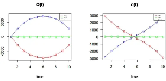
, that is, qis also an arbitrage in a weak sense.

In the fohowing, we show three cases of the trades where the large trader execute a round trip trade, i.e.,

_{\overline{Q}_{1}=\overline{Q}_{T+1}=0}

: $\mu$_{$\varepsilon$_{t}}=1, $\mu$_{$\varepsilon$_{t}}=0, $\mu$_{$\epsilon$_{\mathrm{t}}}=-1

(5)

\mathrm{Q}(\mathrm{t})

\mathrm{q}(\mathrm{t})

2 4 6 8 \mathrm{t}\mathrm{O} 2 4 6 8 \mathrm{f}0

lime time

Figure 1. Remaining Execution Volume

\overline{Q}_{t}

and Execution Volumeq_{t}

(t=1, \ldots, T)

From these graphs, we find that, in the cases$\mu$_{$\varepsilon$_{t}} \neq 0, the large trader is able to increase the

expected utility of the final wealth by starting from

\overline{Q}_{1}

=0_{. Therefore, if}_{$\mu$_{$\varepsilon$_{\mathrm{t}}}} _{\neq 0, then there exist}

round trip trades which satisfy an arbitrage in a weak sense.

4.2 Comparative Statics

4.2.1 The Effect of Risk Aversion

First, we show the following three cases: R=0.001, R=0.5_{, and}R=1.

\mathrm{Q}\langle \mathrm{t}|

1 2 4 6 8 10 time

\mathrm{q}(\mathrm{t})

2 4 6 8 10 ガme

\overline{Q}_{t}

and Execution Volumeq_{t} (t=1_{i}\ldots, T)

As these graphs show, the more risk averse the large trader is, the faster he or she executcs.

(6)

4.2.2 The Effect of$\alpha$_{t}

Next, we see the execution volume of the three cases: $\alpha$_{t}=0.01, $\alpha$_{t}=0.5, and$\alpha$_{t}=1.

\mathrm{Q}\langle \mathrm{t})

1 2 4 6 8 10 time

\mathrm{q}(\mathrm{t})

2 1 1 2 4 6 8 10 time

\overline{Q}_{t}

(t=1, \ldots, T)

These graphs illustrate that the faster the price reverses, the more the large trader tends to execute at the beginning and at the end of the trading.

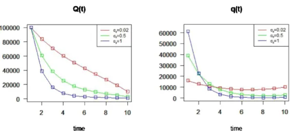
4.2.3 The Effect of_{$\sigma$_{$\varepsilon$_{t}}}

We show the three cases: $\sigma$_{$\varepsilon$_{\mathrm{t}}} =0.02, $\sigma$_{\vee \mathrm{t}} =0.5, and$\sigma$_{$\varepsilon$_{t}} =1.

臆

_{\langle \mathrm{t})}

1 2 4 6 8 10 time

\mathrm{q}(\mathrm{t})

2 4 6 8 10 time

\overline{Q}_{t}

(t=1, \ldots , T)

These graphs ihustrate that if the variance of the effect of the public news is large, the large trader executes more faster for fear that the execution price will be pushed up by the public information.

(7)

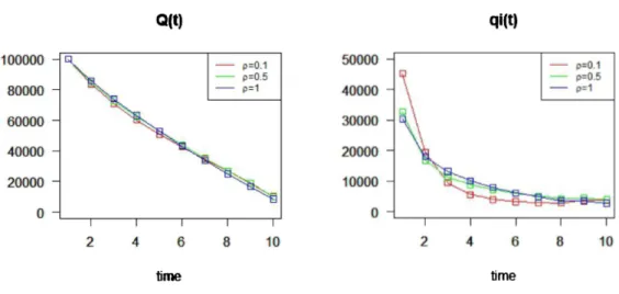
4.2.4 The Effect of the resilience speed

Finally, we demonstrate the three cases: $\rho$=0.1, $\rho$=0.5 , and $\rho$=1.

臆

_{\langle \mathrm{t})}

1 2 4 6 8 10 time

\mathrm{q}\dot{\mathrm{t}}(\mathrm{t})

2 4 6 8 10 time

\overline{Q}_{t}

(t=1, \ldots , T)

We can interpret from these graphs that as the resilience speed increase, the large trader executes their order submit slowly.

5 Conclusion and Future Research

In this article, we derived the optimal execution strategy in the case of single‐large trader, and showed some features of that strategy. However, we did not consider the situation where there are other large traders. Hence, the study on the case of non‐single large trader model would be

remained for our future research.

References

[1] Almgren, R. and N. Chriss: ‘Optimal execution of portfolio transactions,” Journal of Risk, 3, 5‐39, 2000.

[2] Bertsimas, D. and Lo, A. W.: “Optimal control of execution costs Journal of Financial

Markets, 1, 1‐50, 1998

[3] Huberman, G. and W. Stanzl: “Price manipulation and quasi‐arbitrage,” Econometrica, 72,

1247‐1275, 2004.

[4] Kunou, S. and Ohnishi, M.: “Optimal exccution strategy with price impact,” Research Institute for Mathematical Sciences (RIMS) Kokyuroku, 1645, 234‐247, 2010.

[5] Kuno, S. and Ohnishi, M.: “Optimal execution in ihiquid market with the absence of price

manipulation,” Journal of Mathematical Finance, 5, 1‐14, 2015.

[6] Kuno, S., Ohnishi, M., and Shimizu, P.: “Optimal execution with off‐exchange trading,” Jour‐

nal of Mathematical Finance, 7, 54‐64, 2017.

Optimal Execution Strategies with Generalized Price Impact Models (Decision making theories under uncertainty and its applications : the extensions of mathematics for programming)