On the Generation of Wind Waves Relating to
the Shear Flow in Water-A Preliminary Study
著者
Kawai Sanshiro
雑誌名
Science reports of the Tohoku University. Ser.
5, Geophysics
巻
24
号
1/2
ページ
1-18
発行年
1977-03
URL
http://hdl.handle.net/10097/44738
Sci. Rep. TOhoku Univ., Ser. 5, Geophysics, Vol. 24, Nos. 1/2, pp. 1-47, 1977.
On the Generation of Wind Waves Relating to the Shear
in Water — A Preliminary Study
Flow
SANSHIRO KAWAI
Geophysical Institute, Faculty of Science, TOhoku University, Sendai 980, Japan
(Received December 4, 1976)
Abstract: For the study of the phenomena of wind wave generation, measurements
of the surface shear flow and initial waves have been made in a wind wave tunnel, when the wind begins to blow over the still water surface. It is shown that a shear flow
starts in the uppermost thin layer of water at the instance of the start of wind, but
the appearance of waves occurs several seconds later, when the shear flow in water is
still growing. Expecting, from this fact, the initiation of waves by the destabilization
of the shear flow in water, theoretical computations have been made. The result is negative, and it is shown that the initial waves cannot evolve from the destabilization
of the shear flow in water. However, unexpected computational results have been found that the damping factor has a minimum at some value of the wave number.
The wave number of the minimum damping factor ranges from about 2 rad cm-, for
the Reynolds number of the shear flow Re=500 to about 1 rad cm-1 for Re =1500, and
it is slightly smaller than the wave number for waves of minimum phase velocity. On the other hand, it is shown from the experiment that the initial waves are likely to
be waves whose phase velocity is near to the minimum. It is suggested that the shear flow in water may thus bring some effect in selecting the wave number of the initial
waves.
1. Introduction
When the wind begins to blow over a water surface which has been at rest, the following time series of phenomena is seen from detailed observations. A shear flow first starts and grows in the uppermost thin layer of water, and then the appearance of waves follows several seconds later. The initially appearing waves are long-crested and regular, and so they are distinguished from wind waves which are short-crested, irregular, accompanied by forced convections as reported by Toba et al. (1975), and seen after the growth of the initial waves. In this paper much stress is laid on the phenomena of the initial wave generation, among these processes of the generation
and growth of wind waves.
In theoretical works about the mechanism of generation and growth of wind waves, Phillips-Miles combined mechanism (Phillips, 1966) is well known. The theory postulates that, at an earlier stage of the process of the generation and growth of wind waves, Phillips' resonant mechanism is dominant. However, with the experimental study including the measurement of turbulent structure of wind, Plate et al. (1969) showed that the characters of the initial waves could not be explained by the resonant mechanism.
recently reported an experimental study on the process of generation and growth of wind waves by use of methods of microwave scattering. Since experimental studies on temporal growth of wind waves have been scarce, this study is interesting. However, the relation between their observational results and the time series of phenomena stated in the first part of the present section is not necessarily clear, since their direct observational quantities were not the time series of phenomena including the water surface elevation, but the growth rate of power spectral density of wind waves for component waves of certain wave numbers. In relation to these results, Valenzuela (1976) computed the growth rate of wind waves with a coupled shear flow model, or the modified Miles' model. However, since the model was based on the assumption that the mean field of flow is steady, as Miles' model, he could not explain the phenomena that the initial waves are generated a certain moment later from the start of wind.
The shear flow started by wind is a growing flow with time, as reported by Kunishi (1957), and also as shown by our experiment described in the succeeding section. If the growing shear flow destabilize itself hydrodynamically at a certain instance, it is expected that the instance corresponds to the critical time of the generation of the initial waves, or in other words, the generation of the initial waves is caused by the instability of the shear flow in water. At this point it should be noted that an important theorem called as the semicircle theorem was given by Howard (1961) for parallel flows between two rigid walls, and was extended to parallel flows with a free surface by Yih (1972). The theorem says that a necessary condition for the flow to be unstable is that the phase velocity cr of the waves resulted from the instability fulfills the relation uni.<"c in -- max, where umin and umax are the minimum and the maximum velocities of the flow, respectively. On the contrary, our experimental results shown later fulfill the relation cr>uma.. With this fact, the semicircle theorem may lead to a conclusion that the initial waves are not generated as a result of instability of the shear flow in the uppermost thin layer of water. However, the semicircle theorem was derived for inviscid fluids, and the phenomena of wave genera-tion take place at the water surface itself, that is the very boundary of the water, where the viscosity may play a crucial role. Consequently, the above mentioned new mechanism is still conceivable.
In the present paper we will describe firstly our experiment on the shear flow and the initial waves generated by wind, and secondly the theoretical analysis for the test of the new mechanism of generation of the initial waves.
2. Experiment
A pioneering experimental study on the growth of the wind driven shear flow at the uppermost water surface was performed by Kunishi (1957, 1963). His experiments using aluminum powder methods showed that the velocity profile u(y) of the shear flow, where u is the horizontal velocity and y the vertical coordinate taken positive upward from the surface, coincides with the formula,
GENERATION OF WIND WAVES RELATING TO THE SHEAR FLOW IN WATER 3
u(Y)
= e-$2 +177r e(1+00 , (2.1)
which is derived theoretically for the horizontally homogeneous laminar flow in a semi-infinite space exerted by a constant stress at the surface, with an assumption that the pressure gradient is sufficiently small. In the formula the error function 45(e) is defined as
2 ce)
e-.2 dx , (2.2) 117r 0
and the velocity u0 at the surface and the dimensionless coordinate e are defined as
140 V7r pV
2 T .1/t
(2.3)and
(2.4) 2 i/
vt
respectively, and where To is the wind stress which is assumed to be constant, p the density of water, v the kinematic viscosity of water, and t the time measured from the start of wind. However, since the wind speeds used in his experiment were too low to generate wind waves even in the condition that the wind continued to blow long enough, we have performed another experiment for higher wind speed conditions, aiming at the study of the relation of the shear flow and the generation of initial waves.
The experiment was made with a wind wave tunnel of 15 cm wide and 455 cm long. Wind speeds used in the experiment were 4.0, 6.2 and 8.6 m sec-1 in the mean
value in the tunnel section. Wind profiles were measured by a system of a Pitot-static tube and a manometer. The fetch of observation was 2.85 m.
When the wind speed is higher, the onset of initial waves occurs faster, and the depth of the shear flow at the critical time of initial wave generation becomes thinner as conceived from (2.4). Consequently, we have to have measured the distribution of velocity in the thinner shear layer than Kunishi's. As it is hard to insure the accuracy of depth measurement with aluminum powder methods in such a thinner layer, a classified-size particle method was adopted as follows.
As tracers, polystyrene particles were used. The mean specific weight of the particles was 0.99, and they contacted the water surface almost at one point. The speed of each particle approximately represents the speed of water at the depth of the center of the particle. In order to measure the profile of the shear flow, they were sorted into six classes by their sizes. The mean diameter of each class was 0.33, 0.53, 0.73, 1.03, 1.53 and 1.93 mm, respectively, and their maximum deviation was 0.05 mm. The movement of these particles was filmed by a I6-mm cinecamera from the top, and the instantaneous speed of the particles was determined from the distance of the particles moved in the adjacent two frames. The interval of the frames was about I/40 sec. A detailed description of the treatment of these particles,
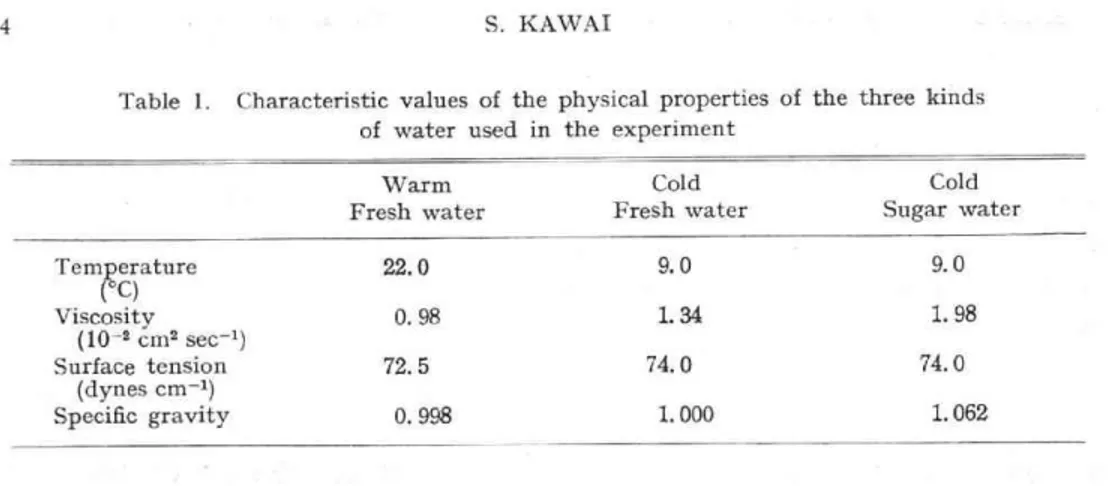
specifica-Table 1. Characteristic values of water
of the physical properties of the used in the experiment
three kinds Warm Fresh water Cold Fresh water Cold Sugar water Temperature (°C) Viscosity (10-2 cm2 sec-1) Surface tension (dynes cm-1) Specific gravity 22.0 0. 98 72. 5 0. 998 9.0 1.34 74.0 1. 000 9.0 1.98 74.0 1.062
tions of the camera and the wind wave tunnel was presented by Okuda et al. (1976) with several photographs.
The critical time of the generation of initial waves, their phase velocity and the wave length were obtained from the same cine-pictures, where the initial waves were perceptible through the change of reflection of light at the water surface.
Since the phenomena of the generation of wind waves might be governed by the viscosity of water, as mentioned in Section 1, three waters of different viscosity were used as shown in Table 1. Since the experiments with the warm water, or the lower viscosity water, were performed in summer, and those with the cold water, or the middle and higher viscosity water, were performed in winter, the change of temperature and other properties of water in each experiment was sufficiently small. The higher viscosity water was prepared by dissolving sugar in cold water. The viscosity was measured by an Ostwald type viscosimeter in a thermally insulated water bath, and the surface tension was measured by the drop weight method. It is seen from the table that the dissolved sugar did not affect the surface tension of water, and that there was no significant change in surface tension throughout the experiment.
It should be noted that even in the heaviest water of 1.062 in specific gravity, the property of the particles that they contact the water surface almost at one point did not change. It was likely due to the hydrophilic nature of the particles colored by a kind of dye, as was reported by Okuda et al. (1976).
3. Results of the experiment
Experiments were performed for nine cases of the combination of the three classes of wind speed: 4.0, 6.2 and 8.6 m sec-1, and the three kinds of water as listed in Table 1. Eight cases were analysed, with an exception of one case of the combination of the lowest wind speed and the middle viscosity water. The reason of the exception was that the original cine-pictures were too light for us to distinguish the particle classes accurately, owing to missetting of the iris diaphram.
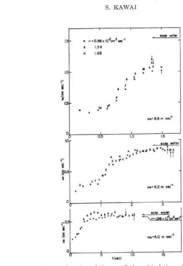
In Fig. 1 are shown the developing processes of the shear flow until the critical time of the initial wave generation is reached for each case. Each point represents an average velocity of five or more particles. The velocity profiles may be approximated by linear functions of depth. From the velocity gradient u0' of the best-fit linear line,
Fig. 1. The
Growth processes of the shear At denotes the time interval
flow of the
until the critical time of initial wave adjoining profiles.
Fig. ' V 5 1 LO ir i ga5 g 0 —O.! ., I g g 0 2. Change of u* as a fi reached. Horizontal arr vertical arrow show the
,•0.98x10⁻²cm2w-I 1.34 1.98 a L5 eL3( verX I Ye' ''. .ter re 11 function of arrows show Ie values of time the 14* at _ soap watt" --\ ..1.98 x faecrese see um.4.0 10 15 thiec)
until the critical time of initial wave generation values of u* estimated from u*a. Points with
the critical time of initial wave generation.
is a
Table 2. Properties of the shear flow at
1 Viscosity of water (10-2 cm2 sec-1) 2 Wind (m sec-9 Observed 3 shear flow 4 Observed initial waves
(cm ato sec-1) d (cm) L (cm) 0.98 1.34 1.. 98 4.0 6.2 8.6 6.2 8.6 4.0 6.2 8.6 12.5 14.5 16.8 13.3 14.6 10.5 10.6 11.3 . 318 . 202 . 138 . 225 .140 . 564 . 297 .191 1.65 1. 97 1.47 1.69 1.55 1.04 2.04 1.41 c (cm sec-1) 32.7 32.8 32.8 30.6 31.4 32.2 29.3 30.0
GENERATION OF WIND WAVES RELATING TO THE SHEAR FLOW IN WATER 7 the friction velocity 74, has been computed using the viscosity v of water through the relation,
u*2 p1401 (3.1) In Fig. 2 is shown the change of u,, as a function of time for each experiment. In the figures for the cases of u„,=-4.0 and 6.2 m sec-1, are also shown values of which have been estimated by use of a relation,
pu*2 pau*a 2 , (3.2) where Pa is the density of air, and u*a is the friction velocity of air, which was determined from the wind profile for a steady state in the restricted condition that the wave formation was suppressed by dissolving some soap in the water. In these cases of lower two wind speeds, it is seen from the figures that the wind stress exerted on the water surface increases with time and reaches to a steady state some time later. Apparently, these unsteadiness of wind stress is caused by the initial unsteadiness of the wind flume with the fun system. However, since the stress values estimated from the shear flow of water approach to steady state values which correspond to those estimated from the wind stress by use of (3.2), it should be concluded that the shear flow in the uppermost layer is controlled by the wind stress and the kinematic viscosity of water. In the case of the combination of u„,-4.0 m sec-1 and v=1.98 X 10⁻² cm' sec-1, the wind stress derived from the wind profile is nearly equal to that on soap water in the same wind speed, as shown in the same figure, since the waves are very small even in the steady state. For the case of u#,=8.6 m sec-1, two differences in the figure from the other wind speeds are seen. Firstly, since the soap water used could not sufficiently suppress the waves, the coincidence of the stresses of the two kinds of estimation could not be found. Secondly, since the onset of the initial waves occur faster, the well-defined steady state could not be found for the values of it,. However, from the trend of the time series of it seems that the initial waves generate just before the stress becomes constant.
the critical time, and of initial waves
Waves
5
for non-shear model
6
Waves for two-layer model
L (cmin) (cm) cmin (cm sec-') L (cmin) (cm) cmin (cm sec-1) C (Lobs) b s) (cm sec-4) 1.72 1.72 1.72 1.72 1.72 1.72 1.72 1.72 35.6 37.6 39.9 36.4 37.7 33.6 33.7 34.4 2. 3 2. 4 2. 4 2. 3 2. 3 2. 1 2.2 2.2 30. 7 30. 2 29. 9 30.0 29.0 31. 1 29.4 28. 5 31. 3 30.4 31.3 30. 6 30.0 33.7 29.4 29.7
It should be noted here that our observational data of the shear flow could not be compared with Kunishi's profile (2.1), by the following two reasons. Firstly, our observation was concerned with the very thin layer in which the profile of the shear flow was essentially linear, while Kunishi's experiment was concerned with macroscopic velocity profiles in the shear flow. Secondly, since the duration of the unsteady wind stress occupied too long part in the time between the start of the wind and the critical time of the initial wave generation, the condition of the constant wind stress, which was supposed in deriving (2.1), and which was obtained for very weak wind speeds by Kunishi, was not fulfilled for our experments of higher wind speeds.
In Table 2 are shown the properties of the shear flow at the critical time, and of initial waves. In Column 1 is shown the viscosity of water, in Column 2 the wind speed, in Column 3 the surface velocity u0 and thickness d of the observed shear flow, the latter being computed from the observed velocity gradient u0' through the relation
= uoid (3.3) and in Column 4 are shown the wave length L and the phase velocity c of the observed initial waves. It is noteworthy that L is an average value of rather scattered values. For comparison, in Columns 5 and 6 are presented the corresponding values computed with two kinds of model. Namely, in Column 5 are shown the minimum phase velocity cmin and its wave length, where the surface velocity u, is taken into account, but where the shear pattern is not taken into account. The cmin was computed by the relation
cmin = comin+uo , (3.4) where comin represents the minimum phase velocity of waves on the still water surface. From the table it is seen that the observed phase velocities are smaller than the minimum phase velocities of the waves for non-shear model, and the model is improper. In Column 6 are shown the minimum phase velocity and its wave length, together with the phase velocity of the wave having the same wave length with the observed one, when the shear flow is taken into account. In computing the values in Column 6, the
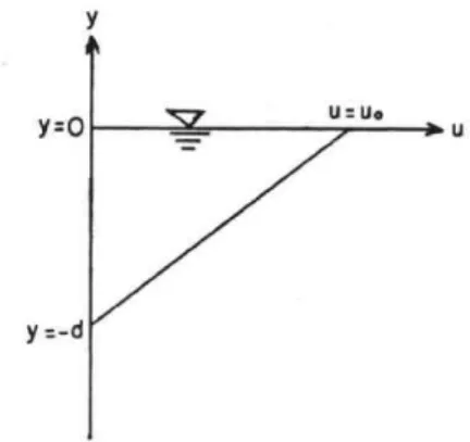
y
Y=0
y =-d
GENERATION OF WIND WAVES RELATING TO THE SHEAR FLOW IN WATER 9 shear flow patterns were approximated by two-layer patterns as shown schematically in Fig. 3. When the theory for multilayer model from Thompson (1949) is adopted to the two-layer model, the relation between the phase velocity c and the angular wave number k is represented as
z3 + a,z2 +(a,a3+ a4) z +a,a4 = 0 , (3.5) where z = — 1 (3.6) /40 1—e--2.a al = 1 + 2 Kd(3.7) 1—e-2" a2 1- 2 K d(3.8) a3 (3.9) Kd co2 (3.10) U0
and co is the phase velocity of the waves on the still water surface. From the table it is seen that the observed wave lengths are not equal to the wave lengths of the waves whose phase velocity are minimum for the two-layer model, but the differences of the phase velocity resulted from the differences of the wave length are small, and these phase velocities for the two-layer model are nearly equal to the observed phase velocities. From this fact, when the above-mentioned scattering of the observed wave length is taken into account, it should be concluded that the observed phase velocities correspond approximately to the minimum phase velocities of the inviscid surface waves on the shear flow. However, since the data is so scanty, more systematic experiments are necessary to establish these interpretation of the results.
So far the discussion is concentrated to the interpretation of the properties of initial waves, and not on the mechanism of the initiation of these waves. As for the latter, from the fact that the maximum velocity uniax of the shear flow or the surface velocity u0 is smaller than the phase velocity of the observed initial waves, the inviscid shear flow instability mechanism cannot explain the initiation of these waves as mentioned in Section 1. In the succeeding sections, we will examine the possibility of the instability mechanism for the viscous shear flow having a free surface.
4. Formulation of the viscous shear flow instability
41 Basic equations
We consider the motion in a vertical plane of an incompressible fluid whose density and kinematic viscosity are p and v, respectively. If x denotes the horizontal coordi-nate on the still surface of water in the direction of a mean flow, and y the vertical
ui+itux+vuy— px+v(u,x+ uyy)
and (4.1)
v,d-uvx+vvy--= —p-lpy+v(v,x+vyy)—g,
where u and v the velocities in the direction of x and y, respectively, g the acceleration of gravity, and the suffixes x, y and t represent differentiation with respect to x, y and t, respectively. The equation of continuity is
ux±vy 0 . (4.2) The dependent variables u, zi and p are expressed as sums of the mean and the perturba-tion values:
U v — V --JTv' and P - p' , (4.3) where capital letters represent mean values and small letters with a prime the perturba-tion values. From the nature of the problem, the mean flow is represented by
U U(Y) and V — 0 . (4.4) The substitution of (4.3) and (4.4) into (4.1) and (4.2), the averaging and the lineariza-tion lead to the equalineariza-tions of molineariza-tion and of continuity for the perturbalineariza-tion flows:
lilt+ Uit' x+v'Uy fi'x+v(it',,x+utyy) , v't+Uv',ppi y+v(vi xx+V'yy)(4.5) and
nix+v'y— 0 , (4.6) respectively. Cross-differentiation of (4.5), considering (4.6), leads to the vorticity equation:
tix-Fv'Uyy T v(-xx+ 'yy) (4.7) where
u'y —v', . (4.8) From the continuity equation (4.6), the stream function IP. may be introduced which satisfies
it' =Iffy and v' = (4.9) and whose form is
y, t) = p( y) exp i(Kx—wt) , colic c , (4.10) where K is the angular wave number and co the angular frequency. Using (4.9) and (4.10), (4.7) leads to the Orr-Sommerfeld equation:
V
(U -C) (pyy-U K29),yy = 2K(.73,1 yy -2K2 pyy + K4.73) • (4.11)
4.2 Boittidary conditions
For a model of two-layer fluids of air and water, boundary conditions at the interface are considered as follows. For the continuity of tangential and normal stresses at the interface
GENERATION OF WIND WAVES RELATING TO THE SHEAR FLOW IN WATER 11
pv(uy+vx) = pav,,(74,0,±vax) (4.12) and
(—fi+2pvvy) — (— pa ±2pav av ay) = T77 , (4.13) respectively, at y =n, where T is the surface tension and the suffix a indicates the value for the air. The continuity of vertical and horizontal velocities at the interface gives v = v a , (4.14) and
it = it, , (4.15) respectively, at y=-77. The kinematic boundary condition is
v nt+unx+vny , (4.16) at y—n. Expanding the conditions from (4.12) to (4.16) around y=0 and neglecting higher order terms, we obtain the following five boundary conditions at the interface for the perturbation quantities:
pv(u' y U yyn x) pava(te ay+ U -Evfi ax) , (4.17) (-p' + +2pvi/ y) — (— P' a+ pap] +2pavav' ay) — T17xx , (4.18)
v' v'a , (4.19)
y7) = a 4- Uayrf, (4.20) and
v' ne+Unx, (4.21) at y =0. When the interface elevation 77 and the perturbation pressure p' with the forms
— exp i(Kx —cot) , (4.22) and
= fi (y) exp i(Kx —cot) , (4.23) are considered, we will have the boundary conditions for 93 in (4.10),
pv(pyy+ Uyy + Op) = Palia(Payy+ Uayy4 K249a) (4.24) (p— pa) KCO2e - 2iK(pvpy— pav away) , (4.25) 99 — 'Pa , (4.26) 97y+ U = Pay Uaye (2.27) and
q) (c—U) , (4.28) at y-0, where
c02 _ g,_1+7.,(p (4.29) From the equation of motion (4.5)
,,v
and the relation is held also for the air. For the continuity of the mean tangential stress at the interface,
pri( I 5, = pavaUay , (4.31) at y=0. At this stage, if we let pal p approach zero, we get finally the boundary condi-tions for water motion at the surface, in the case where there is no air above, as
{(U —c) —3iKv} cpy = y+Kce(U —c)-1-3iKvUy(U Vpyyy , (4.32) and
pyy+U yy(c—U) 19Oc2 = 0 , (4.33)
at --
On the other hand, for the finiteness of motion at infinity,
7) lt.="-0 , (4.34) or q). 0 ; (4.35) at y— —co. 4.3 Nondimensional formulation
The problem considered is to solve the Orr-Sommerfeld equation (4.11) with the boundary conditions (4.32), (4.33) and (4.35). These equations are normalized with the scale velocity u, and the scale length 8, and transformed in nondimensional forms to (U —c)(p((ply ff—Op) — U"9 -1(4.36) _2„.29,,, +
[(U = (U' + K co2(U —c)-1-3iKRe-1U' (U —c)-1)cp —i(KRe)-1q,"' ; y = 0 , (4.37) cp" U" (c —U)-1 (73 + K2q) --= 0; y = 0 , (4.38) and
99 = 9D1 ---- 0; y —co , (4.39) where the prime represents hereafter differentiation with respect to y, and the all variables are nondimensional. In these formulas
c02 (KFr)-1 +1.CW e-1 , (4.40) from the dispersion relation, and the three nondimensional parameters Re, Fr and We are defined by 2 U05P24028( 4.41) Re =Fr0and 'T We -- respectively.
In the present paper, the basic flow pattern is assumed as the form (2.1) and the scale velocity it, and scale length 8 are taken as
2 TO t u(4.42) , 0— V 7C P
GENERATION OF WIND WAVES RELATING TO THE SHEAR FLOW IN WATER 13 and
5 = 21/zit , (4.43) respectively. Although the scale parameters u0 and 5 depend on time, it is assumed that a quasi-steady state is realized at any time.
The problem represented by the equations from (4.36) to (4.39) forms an eigen value problem. When the basic flow pattern U(y), U"(y) and U'(0), and the nondimensional numbers Re, Fr and We are given, the eigen value c can be taken for any wave number K. The eigen value is complex and the sense of its imaginary part ci is important. When and only when ci is positive, the perturbation whose wave number is K is unstable. Consequently, the sense of ci occupies a central part of the problem.
5. Numerical procedure
As the equation (4.36) contains variable coefficients U(y) and U"(y), and the boun-dary conditions (4.37) and (4.38) are of complexity, it is difficult to solve them analyti-cally, and they must be solved numerically. There are several numerical computation schemes for Orr-Sommerfeld equation, as was reviewed by Gersting and Jankowski (1972). We used an orthogonalization method by Betchov and Criminale (1967), which is a modified form of Kaplan's (1964) scheme, and the name of which is from the classification by Gersting and Jankowski (1972). The central technique of the scheme is as follows. Initially an eigen value is assumed, and (4.36) is integrated from y=—co by the method of Runge-Kutta numerical integration, then the dependent
variables such as p are evaluated at y =0. If these values satisfy the surface boundary conditions (4.37) and (4.38), the assumed eigen value proves true. If not, another eigen value is tested, and the iteration is continued until the true one is found.
There are two problems in numerical procedures of the scheme. The first is that we cannot treat y=—cia numerically. This is overcomed by starting the integration from y=y, where U and U" are sufficiently small. Dependent variables such as q at y=ys are taken as the values of the analytical solution which is known from (4.36) if U=U"=0. The second problem is more serious. Although the fourth order differential equation (4.36) has in general four independent solutions, the number of independent solutions is reduced to two when the boundary conditions (4.39) at y--c/3 are taken into account. At y=y, the two independent solutions are started and (4.36) is inte-grated numerically stepwise from y=ys. However, when the numerical integration is performed simply, the independency of the two solutions is broken. Physically speaking, the two independent solutions are viscous solution and inviscid solution, and when Re or K is large, the viscous solution varies largely with y. This variation of viscous solution affects numerically the inviscid solution, and the direct inviscid solution is no more independent of the viscous solution. To overcome this problem, it is necessary to orthogonalize the two solutions in the process of integrating (4.36), although the orthogonalization is not necessary for every steps of numerical integration.
1.03 102 1.01 1.0 0 2.0 Fig. 1.5 .4 1.3 1.2 1.1 0 0 0 4 3.75 Nov. 5 . .. ., ..- 0 0.01 0.02 0.03 0.04 f a 1 h 2 30 as4.0i 0)1 500 a 1 a.i 200 100 I Y. number of stops
4. Change of the value of eigen vector coo at the water surface y=0 depending on the changes of (a) starting point ys and (b) pitch h of the numerical integration for the case of v= 0,98 x 10⁻²cm2sec-1, u.= 1.092 cm sec-1, t= 1.53 sec and K= 4.0 rad cm-1. The ordinate is enlarged in the inserted figures.
• inviscid mode, x viscous mode.
coordinate y s of the starting point of the integration, the interval N0 of the orthogo-nalization and, of cource, the pitch of integration h. As a standard value of these parameters, we took Lys I =3.75, Nor =5, h =0.0075, respectively. However, when Re or IC is large, these standard values are not sufficient to estimate the eigen value accurately. The values of parameters for these cases are decided as that the error of value of po at the surface y=0 is smaller than 0.1% for either of the viscous and inviscid solutions. In Fig. 4 is shown the variation of po for the case of v-0.98 x 10⁻² cm2 sec-1, =1.092 cm sec-1, 1=1.53 sec and K =4.0 .0 rad cm-1, when the parameters y, and h are changed. From the figure it is considered that the values of parameters used are sufficient for required accuracy. For Nor, 50 is sufficient but 5 is used, as the cpu-time of computation did not change largely.
6. Results of computation and discussion
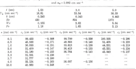
In Table 3 are shown results of the computation for the case of v=0.98 x 10⁻²cm2 sec-1 and it, =1.092 cm sec-1. This case corresponds to the experiment of the com-bination of low viscosity shown in Table 1 and high wind speed of ism=8.6 m sec-1, and in the experiment the initial waves were generated at 1=1.53 sec. Since the correspond-ence between the experimental shear flow pattern and the form (2.1) cannot be verified as was stated in Section 3, the numerical computations have been made also for the cases of higher Reynolds numbers. However, in any case c1 is negative, and from the tendency of ci in relation to Re and K shown in Fig. 5, it seems that there is no eigen value whose imaginary part ci is positive in the vicinity of the computed region in Re-K plane. We may now conclude that the generation of initial waves as described in Sec-tion 3 cannot be explained by the dynamical instability of the shear flow in water itself.
GENERATION OF WIND WAVES RELATING TO THE SHEAR FLOW IN WATER 5.0 4.0 +: 3.0 5 ° 2 .0 1.0 0 .-0.13, 15 0 500 Re1000 1500
Fig. 5. Contour lines of ci in Re-K plane for the case of v=0.98 x 10⁻²cm2 sec-1 and u*= 1.092 cm sec-1. Solid circles represent the points of computation.
Table 3. Computational results for the case of v ---- 0.98x 10⁻² CM" sec-1
and u* =-- 1.092 cm sec-1 t (sec) Elo (cm sec-1) 5 (cm) Re ITTe Fr 1.53 16.81 0.245 420 0. 955 1.18 3.0 23.54 0. 343 824 2.62 1.65 5.0 30.39 0.443 1373 5.64 2.13
,c (rad cm-1) cr (cm sec-1) ci (cm sec-1) cr (cm sec-1) ci (cm sec-1) Cr (cm sec-1) ci (cm sec-1)
0. 1 0. 5 1. 0 2. 0 3.0 3.3 3.7 4.0 10. 0 99. 422 46. 592 36. 093 31.409 31. 180 31.391 31.777 32. 124 40. 983 -0 .308 - 0.171 -0 . 151 -0 . 147 - 0.152 -0 .156 - 0. 160 -0 .163 - 0 .248 99. 799 48. 563 39. 613 36. 413 36.764 38. 007 ---0.228 -0 . 140 -0 .130 - 0 .133 - 0.143 - 0 .156 100. 335 51.405 44.231 42. 221 42. 943 - 0. 186 -0 .123 -0 .119 -0 . 124 - 0. 137
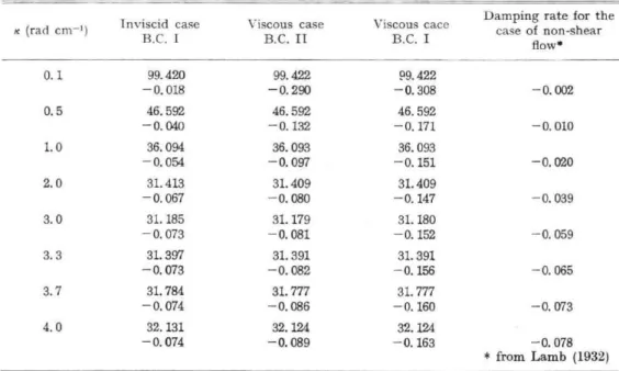
In the rest part of this paper, we will discuss the effect of viscosity, in relation to the results in Table 3. For this purpose, the computations have been made for the case of inviscid fluid having the same shear flow. In this case, the numerical computa-tion is easier, as the orthogonalizing technique is not necessary. It is noteworthy that the surface boundary condition (4.37) contains the information of the shear flow of the air through the relation (4.31), and the resultant term or the third term on the right hand side of (4.37) works in enlarging the damping effect as was pointed out by Keller et al. (1974), although the basic flow pattern used by them was not the same as ours. To discriminate the effect of this term from others, the computation has been made also for the case where this term in (4.37) is neglected. Hereafter this new boundary condition is named as II and the above described standard boundary condition is named as I. Physically, the boundary condition II represents the case that the basic flow is made by the thrust of the floating film at the surface whose rigidity and elasticity are zero. In Table 4 are shown the results of the additional computations, including the standard case listed in Table 3 for comparison.
Table 4. Comparison among computed values of c, and ci for different values of v 0.98 x 10⁻² cm' sec-1, u*= 1.092 cm sec-1 and t=1.53
In each set of values, the upper value represents cr (cm sec-1) and ci (cm sec-1)
conditions. The sec are common.
the lower value
K (rad cm-1) Inviscid case B.C. I Viscous case B.C. II Viscous cace B.C. I
Damping rate for the case of non-shear flow* 0. 1 0.5 1.0 2. 0 3. 0 3. 3 3.7 4. 0 99.420 - 0 .018 46.592 - 0 .040 36. 094 - 0 .054 31. 413 - 0 .067 31. 185 - 0 . 073 31.397 - 0 .073 31. 784 - 0 .074 32. 131 -0 . 074 99.422 - 0 .290 46.592 - 0 . 132 36. 093 - 0 .097 31. 409 -0 .080 31. 179 - 0 .081 31. 391 -0 .082 31. 777 -0 .086 32. 124 -0 .089 99.422 - 0 .308 46. 592 - 0 .171 36. 093 - 0 . 151 31. 409 -0 . 147 31. 180 -0 .152 31. 391 -0 . 156 31. 777 -0 .160 32. 124 - 0 . 163 -0 .002 - 0 .010 - 0 .020 - 0 .039 - 0 . 059 -0 .065 - 0 . 073 -0 .078 * from Lamb (1932)
From the table three facts are noted as follows. Firstly, the phase velocity is determined mainly by the basic flow pattern, or the effects of viscosity and surface boundary condition to it are negligibly small, and it is represented as
CrV , I = CrV, II CrI v, I , (6.1) where suffixes V and Inv represent viscous and inviscid cases, respectively, and suffixes I and II represent the two kinds of boundary conditions. Secondly, even in the shear flow case, the viscosity works as a damping factor, and it is represented as
civ, r ciinv,r+civ,ii • (6.2) Thirdly, there is a minimum in the absolute values of c1, and this fact is different from the case of non-shear flow, in the latter case c1=-2Kv, as was presented by Lamb (1932). Although the number of cases of our computation is limited , it is suggested that the existence of a shear flow in water may bring an effect of selecting the wave number of the initial waves, when they are generated by some mechanism which might be inherent in the coupling with the air flow.
Acknowledgements: The author wishes to express his gratitude to Professor Y . Toba of Tohoku University for his encouragement and discussion , and to Mr. K. Okuda of Tohoku University for his collaboration in the experiment and encouragement , throughout the study. He also expresses his thanks to Dr. F. Sakai of Kawasaki Heavy Industries, Ltd. and Mr. M. Tokuda of Tohoku University , for their kindness in
GENERATION OF WIND WAVES RELATING TO THE SHEAR FLOW IN WATER 17
ing him with useful informations about the computational techniques. The computa-tions in this paper were carried out by NEAC-2200-700 in the Computer Center of
Tohoku University. This study was partially supported by the Grant-in-Aid for Scientific Research, Project No. 942004, by the Ministry of Education.
References
Betchov, R. and W.O. Criminale, Jr., 1967: Stability of parallel flows, Academic Press, 330 pp. Gersting, J.M. and D.F. Jankowski, 1972: Numerical methods for Orr-Sommerfeld problems,
International J. for Numerical Methods in Engineering, 4, 195-206.
Howard, L.N., 1961: Note on a paper of John W. Miles, J. Fluid Mech., 10, 509-512.
Kaplan, R.E., 1964: The stability of laminar incompressible boundary layers in the presence of compliant boundaries, Massachusetts Institute of Technology, Aeroelastic and
Structures Research Laboratory„A.SRL-TR 116-1.
Keller, 1t-.C., T.R. Larson and J.W. Wright, 1974: Mean speeds of wind waves at short fetch, Radio Science, 9, 1091-1100.
Kunishi, H., 1957: Studies on wind waves with use of wind flume (I) On the shearing flow in the subsurface boundary layer caused by wind stress —, Ann. Disas. Prev. Res. Inst., Kyoto Univ., 1, 119-127 (in Japanese).
Kunishi, H., 1963: An experimental study on the generation and growth of wind waves, Disas. Prev. Res. Inst., Kyoto Univ., Bull., No. 61, 4lpp.
Lamb, H., 1932: Hydrodynamics (6th ed.), Cambridge Univ. Press, 738pp.
Larson, T.R. and J.W. Wright, 1975: Wind-generated gravity-capillary waves: laboratory measurements of temporal growth rates using microwave backscatter, J. Fluid Mech.,
70, 417-436.
Okuda, K., S. Kawai, M. Tokuda and Y. Toba, 1976: Detailed observation of the wind-exerted surface flow by use of flow visualization methods, J. Oceanogr. Soc. Japan, 32, 53-64. Phillips, 0.M., 1966: The dynamics of the upper ocean, Cambridge Univ, Press, 261pp. Plate, E.J., P.C. Chang and G.M. Hidy, 1969: Experiments on the generation of small water
waves by wind, J. Fluid Mech., 35, 625-656.
Thompson, P.D., 1949: The propagation of small surface distrubances through rotational flow, Ann. New York Academy of Sciences, 51, 463-474.
Toba, Y., M. Tokuda, K. Okuda and S. Kawai, 1975: Forced convection accompanying wind waves, J. Oceanogr. Soc. Japan, 31, 192-198.
Valenzuela, G.R., 1976: The growth of gravity-capillary waves in a coupled shear flow, J. Fluid Mech., 76, 229-250.