Monetary and Exchange Rate Policy in Malaysia
before the Asian Crisis
著者
Umezaki So
権利
Copyrights 日本貿易振興機構(ジェトロ)アジア
経済研究所 / Institute of Developing
Economies, Japan External Trade Organization
(IDE-JETRO) http://www.ide.go.jp
journal or
publication title
IDE Discussion Paper
volume
79
year
2006-12-01
INSTITUTE OF DEVELOPING ECONOMIES
Discussion Papers are preliminary materials circulated
to stimulate discussions and critical comments
DISCUSSION PAPER No. 79
Monetary and Exchange Rate Policy
in Malaysia before the Asian Crisis
So UMEZAKI*
December 2006
Abstract
This paper provides a case study to characterize the monetary policy regime in Malaysia, from a medium- and long-term perspective. Specifically, we ask how the central bank of Malaysia, Bank Negara Malaysia (BNM), has structured its monetary policy regime, and how it has conducted monetary and exchange rate policy under the regime. By conducting three empirical analyses, we characterize the monetary and exchange rate policy regime in Malaysia by three intermediate solutions on three vectors: the degree of autonomy in monetary policy, the degree of variability of the exchange rate, and the degree of capital mobility.
Keywords: monetary policy, exchange rate, capital control, Malaysia
JEL classification: E42, E58, F41
* Research Fellow, Development Strategies Studies Group, Development Studies
Center, IDE ([email protected])
The Institute of Developing Economies (IDE) is a semigovernmental,
nonpartisan, nonprofit research institute, founded in 1958. The Institute
merged with the Japan External Trade Organization (JETRO) on July 1, 1998.
The Institute conducts basic and comprehensive studies on economic and
related affairs in all developing countries and regions, including Asia, the
Middle East, Africa, Latin America, Oceania, and Eastern Europe.
The views expressed in this publication are those of the author(s). Publication does not imply endorsement by the Institute of Developing Economies of any of the views expressed within.
INSTITUTE OF DEVELOPING ECONOMIES (IDE), JETRO
3-2-2, WAKABA,MIHAMA-KU,CHIBA-SHI CHIBA 261-8545, JAPAN
Introduction
The Asian Crisis triggered wide-ranging and extensive research on the optimal choice of exchange rate regimes in emerging markets (Frankel [1999], Mussa, et al [2000], Williamson [2000], etc.). Discussions over monetary policy rules, such as inflation targeting, have been reactivated as well, focusing on how to enhance the credibility of monetary policy (Bernanke, et al [1999], Taylor [1999], Blejer, et al [2000], etc.). In addition, the debates over capital account liberalization and/or capital controls, which are not separable from the exchange rate and monetary policy, have drawn considerable attention (Eichengreen, et al [1998], Fischer, et al [1998], Edwards [2000], etc.).
A monetary policy regime is defined as an analytical framework which encompasses the three directions of study above. Specifically, a monetary policy regime is characterized by the degree of autonomy in the conduct of monetary policy, the choice of exchange rate regimes, and the degree of international capital mobility. These three conditions can be summarized in the idea of ‘the open economy trilemma.’ A trilemma, in general, is a situation in which, out of three desirable options, at most only two can be pursued. Central banks generally want to retain their autonomy to conduct monetary policy to pursue domestic policy goals. Exchange rate stabilization is regarded as one of the most important policy goals for most central banks. A high degree of international capital mobility is widely recognized as desirable in terms of the optimal allocation of capital. In a textbook world, the choice of monetary policy regimes is simplified to the problem of choosing two out of the three favorable options shown above. However, such a simplification cannot be justified all the time. In reality, many emerging market economies, which have pursued exchange rate stabilization and capital account liberalization, have not addressed the trilemma. For example, before the Asian Crisis, many Asian countries were keeping a nominal anchor by restricting exchange rate movement within a narrow band on the one hand, attempting to retain autonomy in the conduct of monetary policy on the other.
For macroeconomic stabilization, the choice of the optimal monetary policy regime is a very important policy issue. However, the answer to the question is not clear-cut. It depends heavily on the structure and the state of the economy. Therefore, it is crucial to pay enough attention to specific conditions of the economy in question, in order to investigate the optimal choice of monetary policy regimes.
This article provides a case study to characterize the monetary policy regime in Malaysia, from a medium- and long-term perspective. Specifically, we ask how the central bank of Malaysia, Bank Negara Malaysia (BNM), has structured its monetary policy regime, and how it has conducted monetary policy under the regime. In the following sections, we analyze the three conditions which define the monetary policy regime: the monetary policy, the exchange rate policy, and the international capital mobility. It is not possible, of course, to divide these three options, because they are closely related each other. However, organizing the paper along the three vectors is expected to lead to a better understanding on the monetary policy regime in Malaysia.
1. Monetary Policy Autonomy
Central banks in general evaluate the present state of the economy based on the available information at each point of time, and conduct monetary policy to achieve policy goals in the future. Available information includes, for example, monetary and economic statistics up to the previous month. If the available information indicates an inflationary pressure, the central bank would tighten its monetary policy by, for example, mopping up excess liquidity. However, it will take several months for this tight monetary policy to be reflected in the inflation rate. Therefore, it is reasonable to assume that a central bank conducts its monetary policy while taking the time lag into account.
multiple policy goals, by estimating a forward-looking policy reaction function proposed by Clarida, et al [1997, 98]. A policy reaction function defines a policy-setting rule by explaining the movement of policy instruments by the movements of policy goals. Thus, if the estimation results of the policy reaction function satisfy sign conditions with a reasonable stability, we can judge the monetary policy is conducted systematically based on a certain policy rule. In addition, by introducing multiple policy goals into the reaction function, we can examine the relative preference of BNM over possibly conflicting policy goals. Moreover, by adding foreign variables, such as the exchange rate and the foreign interest rate, the degree of monetary policy autonomy can be assessed.
1-1. The Model
A central bank is assumed to set the target of short-term interest rate ( ) during each period. In the baseline model, as shown in (1-1), this target rate is assumed to be dependent on the expected inflation rate and the expected real output. This baseline model regards a nominal interest rate as the only policy instrument and the expected inflation rate and the expected real output as the policy goals, based implicitly on the assumption that the central bank retains autonomy in the conduct of monetary policy.
*
t
i
(1-1) it*=i+β(Ε[πt+k|Ωt]−π*)+γ(Ε[yt+q |Ωt]− yt*)
i is the long-run equilibrium level of the nominal interest rate, π is the inflation rate t+k
from time to , is the information set available to the central bank at time , is the target rate of inflation, is the real output at time
t t+k Ωt t π*
q t
y+ t+ , q is the potential output
at time t , is the rational expectation operator
*
t
y
] [⋅
Ε 1. Since the target rate of inflation is
1 A forward-looking policy reaction function is based on the assumption that the central bank
preemptively conducts its monetary policy in response to the expected value of policy goals. The term ‘forward-looking’ stems from the fact that it takes account of the expected inflation rate and real output in the future (k>0、q>0). This is the significant difference from the standard Taylor rule, in which only current values, i.e. k=q=0, of policy goals are considered (Taylor [1993]). Obviously, a forward-looking
assumed to be constant, denoting the equilibrium level of the real interest rate as r leads to * π + ≡ r i .
Moreover, it is assumed that the central bank cannot adjust the interest rate to the target level instantaneously, because a sudden policy reversal may undermine the market confidence, and it usually takes some time to reach a consensus to change the policy. Accordingly, a partial adjustment process is specified as in (1-2).
(1-2) it =(1−ρ)it* +ρit−1 +υt
t
υ is an independently and identically distributed (i.i.d.) error term. The adjustment speed starting from the interest rate realized in the previous period to achieve the target rate of interest is given as . in general, and the larger the value of ρ , the slower the adjustment speed. The adjustment speed
) 1
( −ρ ρ∈[0,1]
ρ can also be regarded as the parameter, which indicates how strictly the policy rule given in (1-1) is applied. In an extreme case of , the interest rate at time t is determined solely by the interest rate at time t-1, regardless of the target rate of interest. In this case, the policy rule in (1-1) is not working at all. In the opposite extreme case of , the interest rate at time t coincides the target rate of interest, regardless of the interest rate in the previous period. In this case, the policy rule is strictly applied. In general cases of , the interest rate at time t depends both on the interest rate in the previous period and the target rate of interest, and the relative weights are determined by the value of
1 = ρ 0 = ρ 1 0<ρ< ρ . The larger the value of , the slower the adjustment speed. In such a case, the interest rate at time t is dependent more on the interest rate in the previous period than on the target rate of interest. Thus, the policy rule is applied more flexibly than in the case of a smaller value of
ρ
ρ . Substituting (1-1) into (1-2) leads to (1-3).
(1-3) it =(1−ρ)α+(1−ρ)βπt+k +(1−ρ)γxt+q +ρit−1+εt
policy reaction function is a more general specification than the Taylor rule, because the former includes the latter as a special case.
* q t q t q t y y
x+ ≡ + − + is the gap between realized and potential values of real output at time q
t+ . εt is a linear combination of υ and the expectation errors of the inflation rate and the t
real output, and satisfies the orthogonality condition against instrumental variables in estimation (ut ∈Ωt). That is, Ε[εt |ut]=0 is assumed.
Given α r≡ −βπ* and the definition of r , the target rate of inflation can be expressed as
follows: (1-4) 1 * − β α − = π r
The value of indicates the central bank’s stance against inflation (Clarida, et al [1997, p.5]). In a situation where the expected inflation exceeds the target rate of inflation, the central bank would try to calm the future inflation down by raising the target interest rate. Therefore, the sign condition is . Moreover, if
β
0 >
β β>1, the central bank, in response to an inflation expectation, takes a tighter monetary policy so as to keep the real interest rate from falling. This is a policy rule to fight against inflation, which gives priority to price stabilization. On the other hand, if , in response to an inflation expectation, whereas the central bank raises the target interest rate, the increment is not enough to keep the real interest rate from falling. This is a policy rule to accommodate to inflation, in which more attention is paid to the short-term trade-off between inflation and output.
1 0<β<
The value of indicates the central bank’s stance against the stabilization of the real economy. Assume that the central bank conducts monetary policy to stabilize the real economy. If the growth of the real economy outpaces that of the potential output, the central bank would stabilize the real economy by raising the target rate of interest
γ
2. In this case, the corresponding
sign condition is γ>0.
2 However, there are cases in which a central bank gives priority to economic growth at the cost of
However, in a small open economy like Malaysia, it is not appropriate to assume that the monetary policy is conducted based solely on domestic matters3. Indeed, exchange rate
stabilization constitutes one of BNM’s policy goals (Section 2). Additionally, since international capital mobility has been high in Malaysia (Section 3), it is appropriate to assume that foreign interest rates affect Malaysian interest rates through interest rate arbitrage. Therefore, we estimate an extended model given by (1-5) as well. As for , exchange rates and a foreign interest rate will be considered.
t
z
(1-5) rt =(1−ρ)α+(1−ρ)βπt+n+(1−ρ)γxt +(1−ρ)δzt +ρrt−1+εt
Let us consider first a case in which an exchange rate is introduced as an external factor, . When the exchange rate depreciates in comparison with its long-term trend or equilibrium level, the central bank would try to stabilize the exchange rate by raising the target rate of interest. Therefore, the sign condition is if the exchange rate is in a direct expression, or
t
z
0 >
δ δ<0
if it is in an indirect expression4. In the case of δ=0, the central bank does not stabilize the
exchange rate by changing the interest rate.
When we introduce a foreign interest rate as zt, the parameter δ can be interpreted
differently. In this case, the value of δ represents not only a part of the policy rule but also a measure of international capital mobility. If δ=0, the domestic interest rate does not have any partial correlation with the comparable foreign interest rate. The absence of interest arbitrage can be explained by a low degree or a lack of international capital mobility. If capital is mobile internationally so as to produce interest arbitrage, both interest rates would have a positive
3 Clarida, et al. [1997] use the baseline model given by (1-3) to analyze three large economies (G3), the
United States, Japan, and Germany. The analyses on three relatively small economy (E3), the United Kingdom, France, and Italy, which can be reasonably assumed to be under the influence of Germany, the extended model given by (1-5) is used.
4 A direct expression is the price of a unit of foreign currency in terms of domestic currency, for example,
US$1.00=RM3.80; and an indirect expression is the price of domestic currency in terms of foreign currency, for example, RM1.00=US$0.26. Therefore, an increase in the value indicates a depreciation in the case of a direct expression and an appreciation in the case of an indirect expression.
correlation. Thus the sign condition is δ>0. A special case of δ=1 can be interpreted as a case of perfect capital mobility since it implies the interest arbitrage holds perfectly at the margin.
The introduction of foreign factors to the policy reaction function allows us to examine the degree of autonomy of the monetary policy. Suppose first that domestic factors are significant, that is, β>0 and/or γ>0, in the baseline specification. In this case, based on the assumption of a financially closed economy, we can interpret that the monetary policy is conducted based on a certain policy rule5. If the addition of a foreign factor invalidates the policy rule based
on domestic factors ( t z 0 = γ =
β ), we can judge that the central bank lost its autonomy over monetary policy. On the other hand, if domestic factors remain significant after the addition of a foreign factor, the central bank retains its autonomy in the conduct of monetary policy. Additionally, if the foreign factor is not significant, the central bank conducts its monetary policy based only on the domestic factors without any influence of foreign factors. If both domestic and foreign factors are significant, the autonomous monetary policy based on domestic factors is compatible with the monetary policy, which is consistent with foreign factors6.
1-2. Estimation
Due to the nonlinearity of the model, OLS (Ordinary Least Squares) estimates do not retain consistency. Therefore, we estimate the model by GMM (Generalized Method of Moment). Following Clarida, et al [1997], a constant and lagged values (t-1···t-6, t-9, t-12) of explanatory variables are employed as instrumental variables in GMM estimation. In the baseline model, for example, there are 25 instruments whereas the number of parameters to be estimated is only 4.
5 On the contrary, the statistical insignificance of both domestic factors implies the absence of systematic
policy rule.
6 Clarida, et al [1997, p.21] interpret such a situation that the policy interest rate is determined by the
We will test this overidentification by the J test proposed by Newey and West [1987].
The overnight rate of the Kuala Lumpur Interbank Offered Rate (KLIBOR) is used as the policy interest rate. The inflation rate is measured by CPI. The index of industrial production is used as the proxy of real output. The above data is obtained from the BNM Monthly Statistical
Bulletin. The potential output is calculated by a Hodrick-Prescott filtering. We introduce 4
exchange rate variables, the nominal and the real exchange rate against the US dollar, and the nominal and the real effective exchange rate, denoted as NER, RER, NEER, and REER, respectively. The long-term trends of exchange rate variables are also obtained by a Hodrick-Prescott filtering. Note that NER and RER are measured in direct expression, whereas
NEER and REER are in indirect expression. All exchange rate variables are obtained from IMF, International Financial Statistics, CD-ROM. The federal fund rate (USFF), obtained from the
web site of the Federal Reserve Bank, is used as the proxy of the foreign interest rate.
k and p indicates how long the central bank forecasts in the conduct of monetary policy.
Following Clarida, et al [1998], we set k=p=37. The sample spans from January 1988 to August
1998.
1-3. Estimation Results
Table 1 summarizes the GMM estimates of structural parameters. Due partly to the inclusion of the lagged dependent variable, adjusted R-squares are high, around 0.8, in all cases. According to the J-tests, we cannot reject the null hypothesis of overidentification in all cases. This implies that instruments are appropriately selected, in the sense that Ε[εt |ut]=0.
Let us examine first the speed of adjustment parameter ρ , which also measures how strictly the policy rule is applied. In all cases, 0<ρˆ <1 and the sign conditions are satisfied. Wald
7 Clarida, et al [1998] set k=p=1 in their quarterly model. Clarida, et al [1997] set k=12 and p=0, and
tests reject the null hypotheses of ρ=0 and ρ=1 in all cases with very high levels of significance. Thus, the partial adjustment process introduced by Clarida, et al [1997] is appropriate. In all cases, parameter estimates are around 0.9, indicating that the half-lives of the adjustment process are 6 to 9 months. From the viewpoint of the speed of adjustment, these estimates seem to be too high8. It is also possible to interpret these estimates as the policy rule is
applied with a high flexibility.
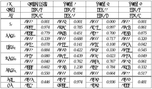
Table 1. Estimation Results of the Policy Reaction Functions
α β γ δ ρ π* R2A/J-test 0.753 1.664 -0.057 - 0.889 0.796 Baseline 0.326 0.002 0.464 - 0.000 3.010 0.925 2.059 1.212 0.174 -0.092 0.921 0.794 NER 0.009 0.336 0.009 0.140 0.000 3.267 0.957 2.185 1.206 0.178 -0.101 0.922 0.794 RER 0.010 0.394 0.007 0.119 0.000 2.760 0.961 2.944 1.072 0.109 -0.335 0.899 0.792 NEER 0.001 0.763 0.085 0.002 0.000 -2.644 0.987 1.966 1.351 0.046 -0.195 0.901 0.794 REER 0.002 0.038 0.431 0.014 0.000 2.246 0.982 -3.465 1.703 0.249 0.917 0.928 0.794 USFF 0.243 0.047 0.011 0.035 0.000 8.846 0.961
Sources: Author’s estimates. For original data, see 1-2.
Notes: Upper cells show the estimates of structural parameters. Lower cells show p-values from Wald tests regarding the null hypotheses that true parameters are zero. As for β, the null hypothesis is β=1. In the last column, upper cells show adjusted R-squared (R2A), and lower cells show p-values from J-tests
of overidentification. In computing the target rate of inflation (π*), we use the average of the ex-post
real interest rate during the sample period, r=2.536.
In the baseline model, the parameter estimate, which represents BNM’s stance against
8 In their analysis on developed countries, Clarida, et al [1997] obtain similar estimates and attribute the
results to the existence of adjustment costs and the fact that central banks are generally unwilling to change interest rates frequently so as to maintain credibility on monetary policy.
inflation, is . This estimate satisfies the sign condition and exceeds 1 significantly. On the other hand, the parameter estimate for does not satisfy the sign condition nor differ significantly from zero. Judging from these results, BNM conducts its monetary policy to fight systematically against inflation, whereas it does not have any systematic policy rule to stabilize the real economy. The target rate of inflation in this setting is 3.01%. The average rate of inflation during the sample period is 3.45% with a standard deviation of 1.04. Thus, we can conclude that the inflation target has roughly been achieved, or that this specification is appropriate enough to derive a reasonable estimate for the target rate of inflation.
664 . 1 ˆ = β γ
Adding the exchange rate against the US dollar, NER or RER, leads to insignificant estimates of , with wrong signs. Moreover, the estimate of δ β becomes small to the extent that Wald tests reject null hypotheses of , though significantly positive. On the other hand, in both cases, the estimate of is significant and positive, indicating that BNM conducts its monetary policy systematically to stabilize the real economy. The target rates of inflation in these cases are around 3%, comparable to that in the baseline specification.
1 > β γ
Adding the effective exchange rates, NEER or REER, leads to different results. The estimates of are significantly different from zero, satisfying the sign conditions. In both cases, we obtain a smaller estimate of than in the baseline case. The estimate of is not different significantly from 1 in the case of NEER, whereas it exceeds significantly 1 in the case of REER. The estimates of satisfy the sign condition in both cases, though not significant in the case of REER. The target inflation rate is negative, , in the case of NEER, and a more reasonable level, , in the case of REER.
δ β β γ 644 . 2 ˆ* =− π 246 . 2 ˆ* = π
As will be discussed in detail in Section 2, BNM has announced officially that it intervenes in the foreign exchange market to stabilize short-term fluctuations in the exchange rate, and the announcement can be confirmed by actual data. Therefore, it seems to be appropriate to add some exchange rate variable in the policy reaction function. However, as presented above, the
estimation results differ considerably by the definition of the exchange rate. Thus, it is important to examine which specification is more appropriate in this specific case for Malaysia. As will be shown in Table 1, since the middle of the 1980s (period 3), the ringgit exchange rate has shown a high correlation with the US dollar; the correlations with the Japanese yen and the Deutsche mark are significant as well. This fact implies that the use of the exchange rate against the US dollar in the policy reaction function may not fully reflect BNM’s policy stance to stabilize the exchange rate. In this respect, the use of effective exchange rates, which are based on a basket of major currencies, seems to be more appropriate. Moreover, the case of REER lead to similar results as in the baseline model, in the respects that β is significantly larger than 1 and that is not significant. The cases of NER, RER, and NEER, on the other hand, lead to different results in both respects. Concerning the target rate of inflation, we have obtained reasonable estimates except for in the case of NEER. Judging from the above findings, the use of REER seems to be the most appropriate among the four alternative definitions.
γ
Finally, let us consider the case in which the federal fund rate is added to the baseline model as a foreign factor. In this case, the estimates of β , , and γ δ are significant, and satisfy the respective sign conditions. Moreover, the estimate of β is significantly larger than 1. In this case, BNM conducts its monetary policy systematically to fight against inflation, to stabilize real output, and to accommodate to the foreign interest rate. A problem in this specification is the estimate of the target rate of inflation, which is unrealistically high. Moreover, a Wald test fails to reject the null hypothesis of δ=1, with a p-value of 0.847. This means that the interest arbitrage has been working fully at the margin, implying perfect capital mobility. Here, we need to take account of the fact that the speed of adjustment is slow as measured by . The target rate of interest based on the policy rule shows a strong correlation with the federal fund rate on a one-to-one basis, the interest rate realized in each period is heavily dependent on the interest rate in the previous period. An important point to note is that the interest arbitrage does
928 . 0 ˆ = ρ
not necessarily hold at each point of time. This, a flexible application of the policy rule, is the very reason why BNM has been able to pursue both the domestic policy goals (β>0 and
0 >
γ ) and the foreign factor (δ>0).
An overall review of Table 1 reveals important implications as follows. Firstly, BNM has conducted its monetary policy based systematically on a certain policy rule. Since the estimates of are significantly positive in all cases, it is reasonable to assert that BNM has paid systematic attention to expected inflation. On the other hand, regarding the policy stance to stabilize real output, no stable result has been obtained. Secondly, the policy rule has been applied rather flexibly. This point can be derived from the results that the estimates of are high, around 0.9. Finally, and most importantly, BNM has conducted its monetary policy based not only on domestic policy goals but also on foreign factors such as the exchange rate and the foreign interest rate. An important point to note is that both the domestic factor (especially
β
ρ
β ) and the foreign factor ( ) are significant in the policy reaction function. That is, even under a high degree of international capital mobility, BNM has conducted its monetary policy in order both to stabilize short-term fluctuations in the exchange rate and to pursue the domestic policy goals.
δ
2. Exchange Rate Policy
After obtaining independence in 1957, the national currency of Malaysia, the ringgit9,
had been pegged to the Pound Sterling. Following the dismantlement of the Sterling Area in 1972, the ringgit was pegged to the US dollar. The ringgit was allowed to float in June 1973,
9 Precisely speaking, the national currency of Malaysia was the Malaysian dollar at this time. The ringgit
was introduced on August 21, 1975. However, for notational simplicity, we use ‘the ringgit’ throughout the paper.
and again pegged to a basket of major currencies in September 1975. Since then to the middle of the 1980s, the exchange rate policy of BNM had focused on the stabilization of the exchange rate against the Singapore dollar. After several speculative attacks, the ringgit was allowed to float more against both the Singapore dollar and the US dollar in the end of 1984. The exchange rate system since then can be classified into a managed floating system. This regime had lasted until July 1997, when BNM gave up to sustain the exchange rate in the wake of the Asian Crisis. Since September 2, 1998, the ringgit has been pegged to the US dollar at US$1.00=RM3.8010.
2-1. Exchange Rates of the Ringgit against Major Currencies
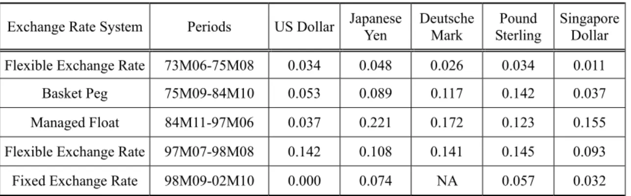
Based on the above classification, Table 2 presents the volatilities of the exchange rate of the ringgit against major currencies. The table provides following implications. Firstly, the exchange rate against the Singapore dollar shows the smallest volatility before the first half of the 1980s. Though the one-to-one conversion against the Singapore dollar was officially abolished on May 8, 1973, as shown in Figure 1, the equivalent rate of exchange had been maintained in practice. Therefore, the flexible exchange rate system between June 1973 and September 1975, and the basket peg system to the middle of the 1980s can be regarded as an exchange rate system characterized as a de facto Singapore dollar peg. By this exchange rate
10 This is a classification of the exchange rate regime based on BNM [1994, 99]. IMF, in its Annual
Report on Exchange Arrangement and Exchange Restrictions, had classified the exchange rate system of the ringgit as a fixed exchange rate system (par value or central rate exist and applied) until its 1973 edition, which refers to the end of 1972; a flexible exchange rate system (exchange rate not maintained within relatively narrow margins) in the 1974 and 1975 editions; a basket peg system (a peg to a composite of currencies) in the editions from 1976 to 1992; and a managed floating system in the editions from 1993 to 1998. Though the timing of the transition to a managed floating system differs from that in this paper, it is very difficult to distinguish a managed floating system from a basket peg system because the composition of the currency basket is, in general, not published. According to Reinhart and Rogoff [2002], which is a comprehensive study to reclassify exchange rate systems, the ringgit is classified into a pegged system against the Pound Sterling until September 1975; a de facto moving band (±2%) system against the US dollar until July 1997; a flexible exchange rate system until September 1998; and a fixed exchange rate system against the US dollar since then to date. Reinhart and Rogoff [2002] refer only to the US dollar and the Pound Sterling, without paying attention to the Singapore dollar. Therefore, their classification until July 1997 does not seem to reflect reality. See Table 2 and Figure 1.
policy, Malaysia imports in effect the basket peg, which Singapore introduced on June 20, 1973. Since the transition to the managed floating system in the middle of the 1980s, the ringgit has gradually depreciated against the Singapore dollar, and the volatility has been enlarged.
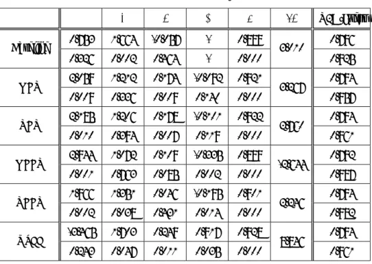
Table 2. Volatility of Ringgit Exchange Rate against Major Currencies
Exchange Rate System Periods US Dollar Japanese Yen Deutsche Mark Sterling Pound Singapore Dollar
Flexible Exchange Rate 73M06-75M08 0.034 0.048 0.026 0.034 0.011
Basket Peg 75M09-84M10 0.053 0.089 0.117 0.142 0.037
Managed Float 84M11-97M06 0.037 0.221 0.172 0.123 0.155
Flexible Exchange Rate 97M07-98M08 0.142 0.108 0.141 0.145 0.093
Fixed Exchange Rate 98M09-02M10 0.000 0.074 NA 0.057 0.032
Sources: IMF, International Financial Statistics, CD-ROM.
Notes: Volatility is defined as the coefficient of variation, which is equal to the ratio of the standard deviation to the mean of the series. Calculated based on the end-of-month figures (AE in the IFS code). Daily data produce similar results.
Secondly, during the period of the managed floating system from the middle of the 1980s to the outbreak of the Asian crisis, the exchange rate volatility against all major currencies except for the US dollar has been enlarged. This fact leads to a widely accepted recognition that the exchange rate system in Malaysia has been a de facto US dollar peg. This point will be discussed further in the next subsection. Thirdly, the transition to a floating exchange rate system in the face of the Asian crisis had increased the volatility against the US dollar but decreased the volatilities against the Singapore dollar and the Japanese yen. This fact implies that the Asian crisis was a common shock in the Asian region. And finally, since the ringgit was pegged to the US dollar in September 1998, the volatility against the other major currencies has been significantly decreased, by importing the stability of the US dollar. Considering the trade
structure of the economy, this is clearly desirable for Malaysia11.
Figure 1. Exchange Rate of the Ringgit against Major Currencies
0.0 1.0 2.0 3.0 4.0 5.0 6.0 7.0 73M01 74M01 75M01 76M01 77M01 78M01 79M01 80M01 81M01 82M01 83M01 84M01 85M01 86M01 87M01 88M01 89M01 90M01 91M01 92M01 93M01 94M01 95M01 96M01 97M01 98M01 99M01 00M01 01M01 02M01
US Dollar Japanese Yen (/100) Deutsche Mark (Euro after 1999) Pound Stering Singapore Dollar
Sources: IMF, International Financial Statistics, CD-ROM.
2-2. The Criteria of the Foreign Exchange Market Intervention
This subsection discusses empirically BNM’s criteria in intervening in the foreign exchange market between September 1975 and June 1997. Specifically, the four major currencies - the US dollar, the Japanese yen, the Deutsche mark, and the Singapore dollar - will be considered as
11 According to the customs statistics, in 2000, the major destinations of Malaysian exports were the
United States (20.5% in total exports), Singapore (18.4%), EU (13.7%), and Japan (13.1%). Major origins of imports were Japan (21.0% in total imports), the United States (16.6%), Singapore (14.4%), and EU (10.8%). These four countries and regions constitute 65.6% of total exports and 62.8% of total imports.
potential benchmarks.
2-2-1. The Model
Following Frankel and Wei [1994], we regressed the percentage change in the ringgit exchange rate on those of the four currencies as an auxiliary estimation. The result shows that the Japanese yen and the Deutsche mark are not significant, though removing the Singapore dollar from the list of explanatory variables makes both currencies significant. However, it is not justifiable to remove the Singapore dollar because the exchange rate policy in Malaysia had focused on the stabilization of the ringgit against the Singapore dollar until the middle of the 1980s, as discussed in the previous subsection. However, it is also difficult to assume that BNM has paid no attention to the Japanese yen and the Deutsche mark. Rather, it seems to be more appropriate to assume that BNM has imported the exchange rate policy in Singapore, which is based on a basket of major currencies. In the following, a casual verification on this discussion will be presented.
Suppose first that Malaysia and Singapore have conducted asymmetric exchange rate policy as shown in equations (2-1) and (2-2). This specification implies that the currency basket for Malaysia consists of the US dollar and the Singapore dollar, and that for Singapore consists of the US dollar, the Japanese yen and the Deutsche mark.
(2-1) M t t t t US SG ML =α +α ∆ +α ∆ +ε ∆ 0 1 2 (2-2) S t t t t t US JP GR SG =β +β∆ +β ∆ +β ∆ +ε ∆ 0 1 2 3
Substituting (2-2) into (2-1) leads to (2-3).
(2-3) M t S t t t t t US JP GR e ML =δ +δ ∆ +δ ∆ +δ ∆ +δ +ε ∆ 0 1 2 3 4 Here, δ0 =α0+α2β0 , δ1 =α1+α2β1 , δ2 =α2β2 , δ3 =α2β3 , and . represents the estimation error, that is, the volatility of the Singapore dollar less a portion which is explained by (2-2). 2 4 =α δ S t e
If the specifications in (2-1) and (2-2) are correct, the estimates of δ obtained from (2-1) i
and (2-2) would coincide with those from (2-3). Thus, a statistical inference on this similarity is useful to evaluate the specifications given in (2-1) and (2-2). Moreover, the estimates of δ i
provide important information on the conduct of exchange rate policy in Malaysia.
In the following empirical investigation, we employ the Swiss franc as the numeraire, following the literature on this subject. All data are obtained from IMF, International Financial
Statistics, CD-ROM.
2-2-2. Estimation Results
A rolling regression of (2-1) on the full sample found two distinct structural changes in November 1978 and August/September 1985. We observe similar structural changes in (2-2) as well, though less significant than (2-1)12. Therefore, we divide the full sample, from September
1975 to June 1997, into three sub-samples: period 1 from September 1975 to October 1978, period 2 from November 1978 to July 1985, and period 3 from September 1985 to June 1997.
Table 3 summarizes main results13. The specification in (2-1) and (2-2) is in general supported
by the results. Wald tests fail to reject the null hypotheses that “the parameter in (2-3) is statistically equivalent to the corresponding parameter in (2-1) and (2-2),” except for the parameters on the Deutsche mark for the full sample (p=0.040) and period 3 (p=0.061). Joint hypotheses that “the five parameters are the same in both approaches” are not rejected in all periods. These findings provide an indirect support for the specification in (2-1) and (2-2).
12 This may imply that exchange rate policies in Malaysia and Singapore have been symmetric to some
extent. That is, the Malaysian ringgit was included in the currency basket to which the Singapore dollar is pegged.
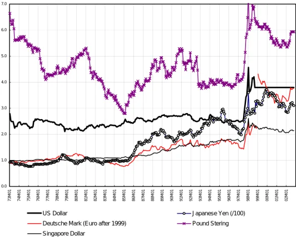
Table 3. Estimation Results
∆ML Full Sample Period 1 Period 2 Period 3
From 75M09 75M09 78M11 85M09 To 97M06 78M10 85M07 97M06 0.001 0.001 0.002 0.001 0.000 0.000 0.001 0.001 δ0 0.398 0.974 0.246 0.785 0.618 0.997 0.415 0.861 0.758 0.779 0.425 0.451 0.711 0.700 0.845 0.875 US: δ1 0.000 0.339 0.000 0.688 0.000 0.717 0.000 0.320 0.081 0.078 0.188 0.141 0.076 0.108 0.064 0.042 JP: δ2 0.001 0.884 0.003 0.422 0.020 0.330 0.078 0.545 0.171 0.080 0.418 0.439 0.041 0.023 0.194 0.049 GR: δ3 0.000 0.040 0.000 0.762 0.494 0.767 0.012 0.061 0.559 0.602 1.145 1.238 0.831 0.784 0.265 0.332 SG: δ4 0.000 0.550 0.000 0.694 0.000 0.664 0.011 0.517 R2A 0.904 0.909 0.943 0.903 DW 1.861 0.446 2.358 0.974 1.742 0.936 1.779 0.481
Sources: Author’s estimates, based on IMF, International Financial Statistics, CD-ROM.
Notes: The left column in each period shows estimation results of (2-3). Upper cells show the estimates of coefficients, and lower cells show the associated p-values. The adjusted R-squared (R2A) and the Durbin-Watson statistic are presented in the bottom of each column. The right column shows the theoretical values based on the estimation of (2-1) and (2-2) in upper cells, and p-values from the Wald test against the null hypotheses that the theoretical values are equal to the estimates from (2-3). The bottom cells of the right columns show p-values from the Wald test against the joint null hypothesis that each of the five parameters is equal between the left and the right columns. P-values in this table are computed based on the Newey and West variance.
Let us turn to the estimate of each parameter. The weight on the US dollar can be divided into two parts: direct response of the ringgit to the US dollar, and indirect response through the Singapore dollar. For instance, the estimate of , which is obtained in the full-sample estimation, can be divided into the direct effect
758 . 0 ˆ 1 = δ 360 . 0 ˆ1 =
α (p=0.001) and the indirect effect 419 . 0 696 . 0 602 . 0 ˆ ˆ2β1 = × =
α 14. Direct responses of the ringgit to changes in the US dollar are
-0.147 (p=0.117) in the first sub-period, 0.174 (p=0.013) in the second sub-period, and 0.628 (p=0.000) in the third sub-period. Because of the specification, changes in the Japanese yen and the Deutsche mark affect the ringgit only though the changes in the Singapore dollar. The
14 The difference stems from the possible specification error and/or estimation error. However, the Wald
weight on the Singapore dollar is given by ˆδ4.
The above analyses provide the following implications on the conduct of exchange rate policy in Malaysia. First, BNM placed more weight on the Singapore dollar than on the US dollar between September 1975 and July 1985. This statement holds even when the indirect effect is taken into account. The weights on the US dollar, including both the direct and the indirect effects, are 0.425 and 0.711 in the first and the second sub-period, respectively. The corresponding weights on the Singapore dollar are 1.145 and 0.831, respectively. However, this situation reversed in the middle of the 1980s. In the third sub-period, the weight on the Singapore dollar has decreased to 0.265, whereas the weight on the US dollar has increased to 0.845. This finding provides support for the widely accepted recognition that, before the Asian crisis, the exchange rate policy in Malaysia was a de facto dollar peg. Second, exchange rates of the Japanese yen and the Deutsche mark have significantly influenced the conduct of exchange rate policy in Malaysia, even though the direct channels are not specified in the model. The de facto weight on the Japanese yen has declined from 0.188 to 0.076 and 0.064 in the three sub-periods. According to the estimation results of (2-2), the weight on the Japanese yen in the currency basket of Singapore has not changed significantly: 0.114, 0.137, and 0.128. Therefore, the decline in the weight on the Japanese yen in the currency basket of Malaysia is attributable to the decline in the weight on the Singapore dollar in the currency basket of Malaysia.
2-3. The Intensity of the Foreign Exchange Market Intervention
This sub-section examines the intensity of the foreign exchange market intervention. The adjusted R-squared (R2A) in Table 3 provides some information on this issue. According to Table 3, R2A exceeds 0.9 in all sample periods. This implies that the foreign exchange market intervention was fairly intense. However, we need some benchmark to evaluate effectively the intensity of intervention.
2-3-1. The Methodology
As measures of the intensity of the intervention, we calculate three indexes proposed by Hausmann, et al [2001、2002] (Hausmann Indexes, hereafter).
The first index, RES/M2, is the ratio of the foreign reserves (RES) to money supply (M2). Under a flexible exchange rate system, this index tends to be small because the central bank does not need to intervene in the foreign exchange market to stabilize the exchange rate. On the other hand, if a central bank does intervene, or has intent to intervene in the foreign exchange market, this index tends to take a larger value.
The second index, RVER, is the ratio of the volatility of the exchange rate to the volatility of the foreign reserves.
(2-4) ) 2 / ( ) ( M RES DEP RVER σ σ = ) (⋅
σ is the mathematical operator indicating standard deviations, and DEP is the rate of depreciation. In order to remove influences of the volatility of the exchange rate to the variable in the denominator, Hausmann, et al [2001] use the average of M2 in the sample period. Under a flexible exchange rate system, RVER tends to be large because the volatility of the foreign reserves is expected to be small. On the other hand, if the central bank actively intervenes in the foreign exchange market, RVER tends to be small because the numerator is expected to be small. In other words, RVER can be regarded as a measure of the intensity of the exchange rate stabilization through direct intervention in the foreign exchange market. The smaller the value of RVER, the more intense the degree of intervention.
The third index, RVEI, is the ratio of the volatility of the exchange rate to the volatility of the policy interest rate.
(2-5) ) ( ) ( i DEP RVEI σ σ =
A central bank can stabilize the exchange rate through the conduct of monetary policy, i.e. by changing interest rates, besides direct intervention in the foreign exchange market. RVEI measures the intensity of this sort of exchange rate policy. If a central bank actively changes interest rates to stabilize the exchange rate, the value of RVEI tends to be small, as obviously shown in the definition. Therefore, the smaller the value of RVEI, the more intense the degree of the commitment.
Hausmann, et al [2001] calculate the above three indexes for 38 countries15, for 1 to 2 years
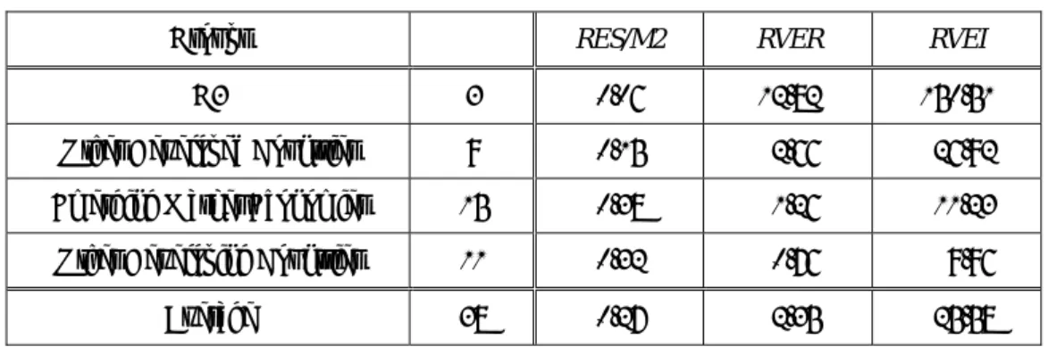
after the Asian crisis. Judging from Table 4, the intensity of the foreign exchange market intervention orders from other developing countries, emerging market economies, other developed countries, to G3 countries, i.e. the United States, Japan, and Germany. This is consistent with our intuitive ordering.
Table 4. Intensity of Foreign Exchange Intervention
Groups # RES/M2 RVER RVEI
G3 3 0.06 12.82 150.51
Other Developed Countries 9 0.15 2.66 26.92
Emerging Market Economies 15 0.38 1.26 11.23
Other Developing Countries 11 0.32 0.76 9.96
Average 38 0.27 2.35 25.58
Sources: Hausmann, et al [2001], Table.1, pp.392-393.
In the following, we present the Hausmann indexes for Malaysia in a time series. Figures in Table 4 can be used as benchmarks to interpret the results. In our calculation, we use the nominal exchange rate against the US dollar and the overnight KLIBOR. The sample period
15 These are the countries classified to have a flexible, managed floating, or crawling/fixed band exchange
rate system by IMF at the end of June 1999, and are included in the BIS database. Thus, Malaysia is not included, because it had already introduced a fixed exchange rate system in September 1998.
spans from January 1975 to August 1998, covering the period when the exchange rate was allowed to float to some extent.
2-3-2. Results
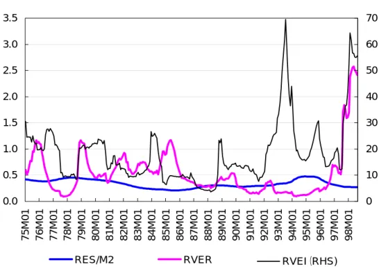
Figure 2 summarizes the Hausmann indexes for Malaysia. All indexes are calculated based on a 24-month period, which ends on the month shown on the horizontal axis of the figure.
RES/M2 changes smoothly within the range between 0.209 and 0.477, with the average of
0.336. This level is roughly equivalent to those of the emerging market economies and the other developing countries, exceeding those of G3 and other developed countries. From the latter half of the 1980s to the middle of the 1990s, RVER for Malaysia was less than 0.5, which was smaller than emerging markets (1.26) and other developing countries (0.76). This implies that BNM’s intervention in the foreign exchange market was more active than central banks in those countries. However, since the latter half of 1996, RVER has sharply increased to a level which is comparable to the average of other developed countries (2.66). Except for the periods of massive capital inflows in the first half of the 1990s and during the Asian Crisis, RVEI for Malaysia has been almost equivalent to the average of emerging market economies (11.23). The hike of RVEI in the first half of the 1990s can be attributed to the sharp appreciation due to the capital inflows, whereas the interest rate stably remained high16. During the Asian crisis, both
RVER and RVEI took high values reflecting the sharply increased volatility in the exchange rate.
On July 14, 1997, BNM announced that it ceased to sustain the exchange rate, and the ringgit was allowed to float. Sharp rises in RVER and RVEI reflect this policy change.
16 High economic growth since the late 1980s generated inflationary pressure, through the expansion of
the domestic demand, the increase in the capacity utilization ratio, and the shortage of labor supply. Accordingly, BNM tightened the monetary policy in the beginning of the 1990s.
Figure 2. Hausmann Indexes 0.0 0.5 1.0 1.5 2.0 2.5 3.0 3.5 75M01 76M01 77M01 78M01 79M01 80M01 81M01 82M01 83M01 84M01 85M01 86M01 87M01 88M01 89M01 90M01 91M01 92M01 93M01 94M01 95M01 96M01 97M01 98M01 0 10 20 30 40 50 60 70
RES/M2 RVER RVEI(RHS)
Sources: Author’s calculation, based on BNM, Monthly Statistical Bulletin, various issues.
The main findings in this analysis are as follows. First, BNM has intervened actively in the foreign exchange market to stabilize the exchange rate of the ringgit. This finding is consistent with the publicly-announced policy that BNM has mitigated short-term fluctuations in the exchange rate and with our preliminary judgment based on R2A in Table 4. Second, the degree of exchange rate stabilization through interest rate policy has been similar to that in other emerging market economies. Third, the amount of foreign reserves held by BNM has been comparable to that in other developing countries, and significantly more than that in developed countries. These findings suggest that exchange rate policy in Malaysia before and during the Asian crisis can be well characterized by “fear of floating” and/or “floating with a life-jacket” (Calvo and Reinhart [2000]).
4. International Capital Mobility
4-1. Capital Mobility and Monetary Policy
Malaysia has long been very open in capital account and foreign exchange transactions because it was a member of the Sterling Area at the time of independence. In 1968, Malaysia received an IMF Article VIII status by liberalizing current account transactions. After the dismantlement of the Sterling Area on June 23, 1972, Malaysia liberalized capital account transactions with countries other than the Sterling Area members on May 8, 1973. This measure expanded further the openness of the Malaysian economy17. Malaysia has been open especially
to transactions in long-term capital, as obvious from the fact that its economic growth since the end of the 1980s depended heavily on inflows of foreign direct investments. However, transactions in short-term capital were regulated when the authorities found it necessary. This sub-section reviews these developments.
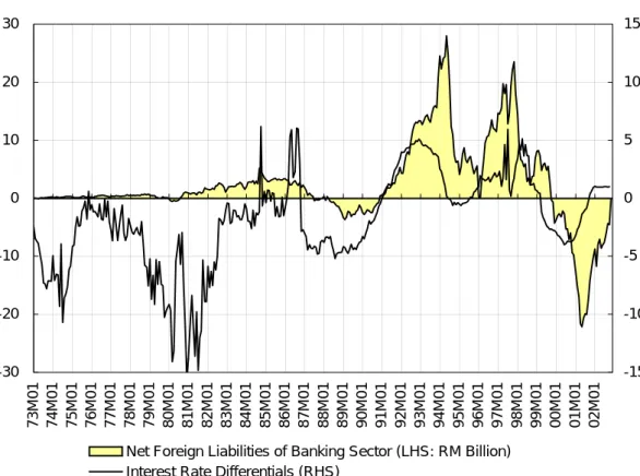
Figure 3 plots the interest rate differentials between KLIBOR and the federal fund rate18, and
net foreign liabilities of commercial banks in Malaysia. Net foreign liabilities of commercial banks capture the movement of capital19. An increase in net foreign liabilities is a result of
capital inflows, and vise versa.
In the 1970s, international capital flows were limited regardless of the large and persistent interest rate differentials in favor of Malaysia. Since the 1980s, the positive correlation between interest rate differentials and net foreign liabilities (capital inflows) has slowly become observable. Since the latter half of the 1980s, this correlation has become more obvious as the magnitude of capital flows was expanded sharply. This change reflects the process through
17 IMF has classified Malaysia as an economy with no restrictions on capital account transactions since its
1974 edition of Annual Report on Exchange Arrangement and Exchange Restrictions.
18 Differentials between other comparable interest rates, such as 3-month interbank rates or discount rates
of treasury bills, show similar movements. Overnight transactions are the most active in the Kuala Lumpur interbank market.
19 Net foreign liabilities are obtained from the balance sheet of commercial banks, which is published in
which Malaysia has been integrated into the international financial market. Of course, interest rate differentials are not the sole factor which cause international capital flows. For example, massive capital inflows after 1991 were caused by the widespread perceptions that the ringgit was undervalued and by international capital flows in general shifting toward emerging markets reflecting expectations on higher returns (BNM [1999], p.289)20. In order to mitigate the
destabilizing effects of such massive capital flows on the domestic economy, various capital controls were imposed when necessary.
Figure 3. Interest Rate Differentials and International Capital Flows
-30 -20 -10 0 10 20 30 73M01 74M01 75M01 76M01 77M01 78M01 79M01 80M01 81M01 82M01 83M01 84M01 85M01 86M01 87M01 88M01 89M01 90M01 91M01 92M01 93M01 94M01 95M01 96M01 97M01 98M01 99M01 00M01 01M01 02M01 -15 -10 -5 0 5 10 15
Net Foreign Liabilities of Banking Sector (LHS: RM Billion) Interest Rate Differentials (RHS)
Sources: BNM, Monthly Statistical Bulletin, various issues.
20 Capital inflows during this period caused a sharp increase in stock prices. The composite index of the
Kuala Lumpur Stock Exchange rose from about 500 in the beginning of 1991 to the then highest of 1314 in May 1994.
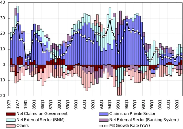
Figure 4 shows the factors affecting the variations in the broad monetary aggregate (M3) in terms of credit allocation. Domestic credits are decomposed into those to the public sector and to the private sector, and foreign assets are decomposed into the changes in the foreign reserves held by BNM and net foreign assets of the banking sector21.
Figure 4. Factors Affecting the Variations in M3 (%)
-20 -10 0 10 20 30 40 1973 1977 1981 85Q1 86Q1 87Q1 88Q1 89Q1 90Q1 91Q1 92Q1 93Q1 94Q1 95Q1 96Q1 97Q1 98Q1 99Q1 00Q1 01Q1 02Q1
Net Claims on Government Claims on Private Sector
Net External Sector (BNM) Net External Sector (Banking System)
Others M3 Growth Rate (YoY)
Sources: BNM, Monthly Statistical Bulletin, various issues.
Notes: Annual data before 1984.
During the recession period in the middle of the 1980s, the growth rate of M3 dropped below 10%, due mainly to the decline in domestic credits to the private sector. Afterwards, M3 showed
21 Different from Figure 3, finance companies, merchant banks, and discount houses are included here, as
well as commercial banks. In addition, note that Figure 4 presents the changes in net foreign assets instead of net foreign liabilities. “Others” include paid-up capital, reserves, and retained profit or losses of BNM and the banking institutions.
a rapid growth in the beginning of the high growth period at the end of 1980s and the beginning of the 1990s because of the rapid expansion of domestic credits. On the other hand, massive inflows of short-term capital caused a decline in net foreign assets in the banking sector since 1991.
Net capital inflows from abroad, which are recorded as either decreases in foreign assets or increases in liabilities on the balance sheet of the banking sector, result in a pressure on the exchange rate of the ringgit for it to appreciate. If BNM sells the ringgit to stabilize the exchange rate, then the same amount of foreign exchange will be added as an asset item, and the same amount of reserves, denominated in the ringgit, will be added as a liability item, on BNM’s balance sheet. On the other hand, the ringgit, which is equivalent to the amount of foreign exchange sold to BNM, will be added as an asset item, reserves held in BNM, on the balance sheet of the banking sector. Since the reserve is a component of the base money, an increase in reserves leads to an increase in money supply by the amount of the increment of the reserve times a relevant money multiplier. In order to avoid increases in money supply through this channel, BNM needs to sterilize the original intervention by selling public bonds, such as TBs and MGS, to the banking sector, to the extent that is equivalent to the increment of reserves. As a result of this sterilized intervention, both BNM’s assets (TBs) and liabilities (reserves) will decrease, keeping the balance unchanged. On the other hand, the banking sector increases its holding of TBs, while decreasing reserves held in BNM. In this way, sterilized intervention, as long as it is conducted effectively, enables BNM to close the channel through which capital inflows increase the money supply.
However, the magnitude of sterilized intervention is restricted by the outstanding amount of public bonds. When BNM conducted massive sterilized intervention in response to massive capital inflows in the beginning of the 1990s, the outstanding amount of official bonds held by BNM decreased sharply from RM 2.68 billion at the end of 1990, to RM 1.61 billion at the end
of 1991, RM 0.56 billion at the end of 1992, and to RM 0.45 billion at the end of 1993. During the period, the fiscal balance improved rapidly and turned to a surplus, and the outstanding amount of public bonds peaked out in 1993. In the face of this situation, BNM issued RM 7.16 billion in Bank Negara Bills (BNBs) in 1993 to continue its sterilized intervention.
This sterilized intervention restrained the growth rate of M3 at around 20% per annum. However, in the fourth quarter of 1993, other massive capital flows came into Malaysia (Figure 3). In response to this, BNM began to consider allowing the ringgit to appreciate by weakening the intervention, in order to discourage capital inflows. After all, BNM dismissed this policy option on the grounds that exchange rate adjustments to deal with the movement of short-term capital are likely to result in overshooting of the exchange rate (BNM [1999, p.289]). Instead, BNM introduced selective foreign exchange controls to repress capital inflows.
3-2. Capital Controls
The foreign exchange controls in Malaysia have been governed by following five principles(BNM [1999, pp.276-277]).
“Export receipt must be brought back and sold to any bank in Malaysia, within six months. However, one could take them out again. The objective is simple, to develop a viable foreign exchange market in Malaysia. The gross flows help to make the market;
Borrowing abroad by residents above a certain limit, require prior approval. Approval is readily given for projects that either generate or save foreign exchange. The rationale is to ensure borrowers have the means to meet external obligations and would not impose a strain on the nation’s reserves. External borrowings are generally not allowed to finance property development for housing and office space in Malaysia and to purchases of shares;
Non-resident controlled companies (NRCCs) who borrow in Malaysia above a certain limit, require prior approval. Approval is readily given to enable the NRCC to finance productive investments in Malaysia provided they bring into Malaysia a reasonable amount of capital of their own for their business ventures; and
For payments abroad, both residents and non-residents were allowed to freely remit abroad their own funds. Approval requirements exist only for residents and only for large
investments. The aim is to encourage the use of the nation’s financial resources for productive purposes within the country.
Selective exchange control measures are policy options to be used on a temporary basis to mitigate the adverse impact of short-term flows on the domestic economy. Such measures are carefully designed and used together with other macroeconomic policies to achieve economic and financial stability. Essentially, such measures would be very specific and well targeted and temporary, to be removed as soon as the objectives of the measures have been achieved. Of importance is such controls would not affect in anyway trade flows and foreign direct investment. Such controls also would not at anytime damage foreign interest in Malaysia”.
Among the above-mentioned principles, the fifth one, which spelled out the possibility of selective capital controls, is of the most interest. Restrictions on inflows of short-term capital in 1993-94 and on outflows of short-term capital during the Asian crisis are examples of this sort of foreign exchange control.
As mentioned above, in the face of the massive capital inflows in the beginning of the 1990s, BNM tried to stabilize both the exchange rate and money supply through sterilized intervention. However, another big wave of capital inflow at the end of 1993 made it difficult for BNM to pursue the goals in the same way. Ultimately, BNM introduced the following measures to repress the inflow of short-term capital(BNM [1999], pp.289-291):
“Expanding the eligible liabilities (EL) base of the banking institutions for the computation of the Statutory Reserve Requirement (SRR) and the Liquidity Requirement to include all inflows of funds abroad, with effect from the base period 16-31 January 1994.
Imposition of limits on non-trade related (after allowing for trade related inflows or for direct investment in Malaysia) outstanding net external liabilities of banking institutions from 17 January 1994. ... This limit was lifted on 20 January 1995.
Restriction on sales of short-term monetary instruments to non-residents with effect from 24 January 1994. The restriction applied only to instruments deemed to be monetary policy instruments used by BNM to influence liquidity in the market. Effective February 1994, the restriction also included private debt securities ... with remaining maturities of one year or less ... The restriction was lifted on 12 August 1994. ...
institutions held in non-interest bearing vostro accounts, effective 2 February 1994. These funds are to be replaced in a designated non-interest bearing account maintained at BNM. ... When the balances maintained in these accounts returned to a more reasonable level, these funds were no longer subjected to the SRR and liquidity requirements with effect from 16 May 1994. ...
Commercial banks were not permitted to undertake non-trade related swaps (including overnight swaps) and outright forward transactions on the bid side with foreign customers beginning 23 February 1994. However, the commercial banks were allowed to undertake swaps or outright forward transactions with foreign customers to hedge their trade related foreign exchange contracts transacted with non-bank domestic customers. This measure was intended to prevent offshore parties from establishing a speculative long ringgit forward position at a time when the ringgit was perceived to be undervalued. This measure was subsequently lifted with effect from 16 August 1994”.
By the third quarter of 1994, net capital flows turned to surplus, and the net foreign assets of banking institutions began to increase. Accordingly, the growth rate of money supply slowed down in the opposite direction through the multiplier process. The year-on-year growth rate of M3 peaked out in the first quarter of 1994 with a high of 29.0%, and sharply declined to 7.8% in the first quarter of 1995 (Figure 4). Under these developments, restrictions on capital inflows, most of which were imposed in the beginning of 1994, were lifted step by step.
However, the growth rate of M3 rose after the second quarter of 1995. Different from the episode in the early 1990s, the growth of M3 at this time was driven mainly by the increases in domestic credits instead of increases in capital inflows. Then, following the outbreak of the Asian crisis, domestic credits shrank sharply, and the M3 growth as well.
By June 1997, portfolio capital had already begun to flow out of Malaysia. The sudden depreciation of the Thai baht following the flotation in July 1997 triggered full-scale speculative attacks on the ringgit. By April 1998, massive capital outflows had hiked the interest rate on the ringgit-denominated deposits in the offshore market in Singapore as high as 30%. Since the Malaysian economy was already in a serious recession at that time, it was very difficult to raise domestic interest rates to discourage capital outflows.
Finally, Malaysia introduced a set of capital control measures directly to stop capital outflows on September 1, 199822. The main components were; (1) imposition of a 12-month holding rule
on the repatriation of funds in External Accounts; (2) control on the transfer of funds in the External Accounts to immobilize trading of the ringgit offshore; (3) control on ringgit-denominated loans to non-residents; and (4) limiting the amount of ringgits that could be imported or exported and the amount of foreign currency that could be exported. On the other hand, BNM aggressively and repeatedly made public announcements that current account transactions and foreign direct investments were not controlled at all. On the next day, September 2, a fixed exchange rate system was introduced at US$1.00=RM3.80.
The control on short-term capital outflows was replaced by a repatriation levy on portfolio funds on February 15, 1999, partly due to the fact that the capital outflows had lost the impetus. In addition, the authority recognized that a gradual liberalization was advisable to avoid a sudden release of capital, which was scheduled on September 1, 1999, 12 months after the imposition of the control. Afterwards, the repatriation levy was further liberalized on September 21, 1999, and subsequently lifted with effect on May 2, 2001.
Concluding Remarks
This paper has analyzed the monetary policy, the exchange rate policy, and capital controls in Malaysia based on a unified framework: the open economy trilemma. This section summarizes main findings of the paper, and draws some policy implications.
Section 1 investigated the operation of monetary policy by estimating forward-looking policy
22 The imposition of capital controls in Malaysia has become the focus of worldwide attention. Among a
bulk of studies, Zainal-Abidin [2000], Dournbusch [2001], Kaplan and Rodrik [2001], Meesook, et al. [2001], Athukorala [2001a,b], and Yusoff [2002] may be good references.
reaction functions following Clarida, et al [1997]. The main findings include; (1) BNM has conducted monetary policy based on a certain policy rule; (2) the policy rule has been flexibly applied; and (3) the policy rule depends not only on domestic factors such as inflation rates and real output, but also on foreign factors such as the exchange rate and the foreign interest rate. The third finding implies that, despite the high degree of capital mobility, BNM had successfully pursued two seemingly incompatible policy goals, namely the stabilization of the exchange rate and inflation.
The open economy trilemma postulates that autonomous monetary policy is not consistent with exchange rate stabilization under perfect capital mobility. More generally, according to Tinbergen’s Theorem, which states that in order to achieve distinct policy goals the number of independent policy instruments must be equal to or exceed the number of policy goals, it is impossible to pursue autonomous monetary policy and monetary policy which is consistent with foreign factors at the same time, when only one policy instrument, the interest rate, is available to the central bank. However, the results shown above are not consistent with these propositions. Let us consider here a possible explanation for this disagreement.
The idea of the open economy trilemma is based on the Mundell-Fleming model, which assumes perfect capital mobility. Perfect capital mobility implies that interest rate arbitrage holds at any instant. Therefore, in a small economy with a fixed exchange rate system, monetary policy is ineffective because the domestic interest rate instantaneously converges to the foreign interest rate. In the case of Malaysia, apart from the periods of temporal capital controls, international capital mobility has been restricted only to a limited extent. However, it should be noted that interest arbitrage does not hold all the time due to the imperfect substitutability of financial assets, imperfect information, and/or the existence of transaction costs23.
23 For example, in their empirical analysis on South Korea, Thailand, Malaysia, and Japan, Norrbin, Li,