THE DEVELOPMENT OF A SPECTROPHOTOMETRIC
METHOD USING FUZZY THEORY
SORANUT KITTIPANYANGAM
A THESIS SUBMITTED IN PARTIAL FULFILLMENT OF THE DEGREE
OF DOCTOR OF MATERIAL SCIENCE AND PRODUCTION
ENGINEERING
FUKUOKA INSTITUTE OF TECHNOLOGY
ACADEMIC 2019
i
Contents
Figure contents ... iii
Table contents... v
Abstract ... vi
Acknowledgments ... vii
1. Introduction ... 1
1.1. Spectrophotometric method ... 1
1.2. Previous multi-component spectrophotometric method ... 1
1.3. Application of multi-component spectrophotometric method ... 2
1.4. Suggestion and contribution in this research ... 2
2. Spectrophotometric method analysis ... 4
2.1. Concentration calculation by light absorbance ... 4
2.1.1. Light absorbance ... 4
2.1.2. Lambert’s law ... 5
2.1.3. Beer’s law ... 7
2.1.4. Beer-Lambert’s law ... 9
2.1.5. Coefficient of determination ... 10
2.1.6. Linear regression analysis ... 11
2.1.7. Multicomponent ... 12
2.2. Comparison of the multicomponent analysis ... 13
2.2.1. Simultaneous equation method ... 13
2.2.2. Derivative spectrophotometry ... 14
2.2.3. Absorb ratio method ... 17
2.2.4. Derivative ratio spectra method ... 21
2.2.5. Double divisor ratio spectra derivative method ... 23
2.2.6. Successive ratio-derivative spectra method ... 26
2.2.7. Isosbestic “isoabsorptive” point method ... 28
2.2.8. Absorptivity factor method ... 28
2.2.9. Q-absorbance ratio method ... 30
2.3. Comparison of the previous spectrophotometric method ... 31
2.4. Deviation of the Beer-Lambert’s law ... 34
2.8.1. Real deviation ... 34
2.8.2. Chemical deviation ... 34
ii
3. Suggestion of the novel spectrophotometric method ... 40
3.1. Analysis of the nonlinear approximation method ... 40
3.1.1. Polynomial regression analysis ... 41
3.1.2. Linear interpolation ... 42
3.1.3. Comparison of the nonlinear approximation ... 43
3.2. Analysis of the proposed spectrophotometric method in the pure solution ... 45
3.3. Analysis of the proposed spectrophotometric method in the multi-component solution ... 47
3.3.1. Fuzzy preparation process ... 52
3.3.2. Fuzzy analysis process ... 57
3.4. Design of the fuzzy set ... 60
4. Comparison of spectrophotometric method between the proposed method and the previous method ... 66
4.1. Comparison in the case of the pure solution ... 66
4.2. Comparison in the case of the multicomponent solution ... 68
4.3. Experiment ... 77
4.3.1. Experimental setup ... 77
4.3.2. Experimental result... 80
5. Discussion and conclusion ... 83
5.1. Discussion... 83 5.2. Conclusion ... 83 5.3. Future study ... 85 Reference ... 87 Appendix ... 92 WPA CO 7500 Colorimeter ... 92
iii
Figure contents
Figure 2.1. Effect when the light goes though the solution. ... 4
Figure 2.2. Relationship between transmission and absorbance when the path length increases. ... 5
Figure 2.3. Relation between the path length and the transmittance. ... 6
Figure 2.4. Relation between the path length and light absorbance. ... 6
Figure 2.5. Relationship between transmission and absorbance. ... 7
Figure 2.6. Relation between the transmittance and concentration. ... 8
Figure 2.7. Relation between the light absorbance and concentration. ... 8
Figure 2.8. Light absorbance of red solution by many wavelengths of the light source. ... 10
Figure 2.9. Ideal light absorbance. ... 11
Figure 2.10. Design of linear function that is the relation between the concentration and the light absorbance.12 Figure 2.11. Process of the simultaneous equation method. ... 14
Figure 2.12. Example light absorbance. ... 14
Figure 2.13. First order derivative of example light absorbance. ... 15
Figure 2.14. First order derivative light absorbance of the mixture solution when the concentration of component y increase. ... 16
Figure 2.15. Amplitude of the first derivative at the zero-crossing when the light absorbance of component x is peak of the curve in zero order. ... 16
Figure 2.16. Process of the derivative method. ... 17
Figure 2.17. Example light absorbance for the absorb ratio method. ... 18
Figure 2.18. Ratio between the light absorbance of component x, component y and mixture and standard of component x. ... 18
Figure 2.19. Light absorbance ratio between the mixture solution and standard solution of component x when concentration of the component y increases. ... 19
Figure 2.20. Difference of the light absorbance ratio (𝐴𝑥+𝐴𝑦 𝐴𝑥0 ) between wavelength 1 and wavelength 2 when the concentration of component y increases. ... 20
Figure 2.21. Process of the absorbance ratio method... 20
Figure 2.22. Derivative of the ratio of the light absorbance from Figure 2.18. ... 22
Figure 2.23. Process of the derivative ratio method. ... 22
Figure 2.24. Light absorbance of 3 components and the mixture solution of 3 components. ... 24
Figure 2.25. Derivative ration light absorbance in the case of 3 components from figure 2.24. ... 25
Figure 2.26. Process of the double divisor ratio spectra derivative method. ... 26
Figure 2.27. Process of the Successive ratio – derivative spectra method. ... 26
Figure 2.28. Light absorbance in many spectra of x, y and mixture solution between x and y the concentration of x and y is half of one concentration in ratio 1:1. ... 28
Figure 2.29. Absorptivity factor point. ... 29
Figure 2.30. Process of the absorptivity factor method. ... 29
Figure 2.31. Process of the Q-absorbance ratio method. ... 31
Figure 2.32. Deviations from the Beer’s law. ... 34
Figure 2.33. Light absorbance of phenol red. ... 35
Figure 2.34. Transformation of the molecule of the phenol red. ... 35
Figure 2.35. Light absorbance by 2 wavelengths when the molar absorptivity of one wavelength is changed. . 37
Figure 2.36. Change of the molar absorptivity per unit change in the wavelength. ... 38
Figure 2.37. Deviated light absorbance of 2 wavelengths. ... 38
Figure 2.38. Case of stray radiation excepting the case of instrument. ... 39
Figure 3.1. Linear function by linear regression analysis. ... 40
Figure 3.2. Concentration calculated by polynomial regression analysis. ... 42
iv
Figure 3.4. Concentration calculated by linear interpolation. ... 43
Figure 3.5. Comparison of the nonlinear approximation. ... 44
Figure 3.6. Comparison of the nonlinear approximation in real deviation case. ... 44
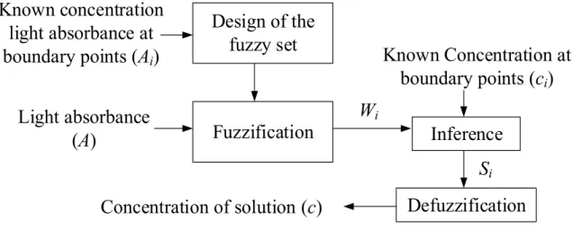
Figure 3.7. Process of the fuzzy theory to calculate the concentration of solution. ... 45
Figure 3.8. Coefficient of the known concentration. ... 46
Figure 3.9. Fuzzy set in the case of the pure solution. ... 47
Figure 3.10. Bilinear interpolation. ... 48
Figure 3.11. Bilinear interpolation (contour graph). ... 48
Figure 3.12. Boundary points of the mixture solution (contour graph). ... 49
Figure 3.13. Calculation of the additional boundary points (contour graph). ... 50
Figure 3.14. Process of the proposed method in 2-component solution case. ... 50
Figure 3.15. Boundary points in the function of the concentration of component x. ... 51
Figure 3.16. Boundary points in the function of the concentration of component y. ... 51
Figure 3.17. Calculation of the concentration of component x at additional boundary points... 53
Figure 3.18. Calculation of the concentration of component y at additional boundary points... 54
Figure 3.19. Flow of the fuzzy preparation process. ... 55
Figure 3.20. Fuzzy set of the fuzzy preparation process. ... 55
Figure 3.21. Additional boundary points calculated by the fuzzy preparation process (contour graph)... 56
Figure 3.22. Calculation of the concentration of component x. ... 57
Figure 3.23. Calculation of the concentration of component y. ... 58
Figure 3.24. Flow of the fuzzy analysis process. ... 59
Figure 3.25. Fuzzy set of the fuzzy analysis process. ... 59
Figure 3.26. Example input light absorbance. ... 60
Figure 3.27. Simulation of the increase of the boundary points without movement of position. ... 61
Figure 3.28. Simulation of the movement of the boundary point positions without change of the number of boundary points... 62
Figure 4.1. Possible concentration case which the concentration of the component is not minus (𝑐𝑥, 𝑐𝑦) (contour graph). ... 65
Figure 4.2. Function calculated by linear regression analysis. ... 67
Figure 4.3. Function calculated by the proposed method. ... 67
Figure 4.4. Comparison of average error by linear regression analysis and the proposed method. ... 68
Figure 4.5. Light absorbance of the 1st detector. ... 69
Figure 4.6. Light absorbance of the 2nd detector. ... 69
Figure 4.7. Calculated concentration of the component x by the simultaneous equation method. ... 72
Figure 4.8. Calculated concentration of the component y by the simultaneous equation method. ... 72
Figure 4.9. Calculated concentration of the component x by the absorbance ratio method. ... 73
Figure 4.10. Calculated concentration of the component y by the absorbance ratio method. ... 73
Figure 4.11. Calculated concentration of the component x by the proposed method. ... 74
Figure 4.12. Calculated concentration of the component y by the proposed method. ... 74
Figure 4.13. Calculated concentration of component x by 5 known concentration data. ... 75
Figure 4.14. Calculated concentration of component y by 5 known concentration data. ... 75
Figure 4.15. Average error of the concentration of the component x. ... 76
Figure 4.16. Average error of the concentration of the component y. ... 76
Figure 4.17. 1st experiment of the mixture solution between red component and green component. ... 79
Figure 4.18. 2nd experiment of the mixture solution between red component and blue component. ... 79
v
Table contents
Table 2.1. Comparison of the previous spectrophotometric method in case of the calculation of concentration
of one component in 2-component solution. ... 33
Table 2.2. Comparison of the previous spectrophotometric method in case of the calculation of concentration of two components in 2-component solution. ... 33
Table 3.1. Ideal known concentration light absorbance of the 1st detector (𝐴 𝑖,𝑗,1𝑠𝑡). ... 49
Table 3.2. Ideal known concentration light absorbance of the 2nd detector (𝐴 𝑖,𝑗,2𝑛𝑑). ... 49
Table 3.3. Value of the variables in additional boundary points... 56
Table 3.4. Average error of concentration (increase of boundary points). ... 61
Table 3.5. Position of the boundary points in the 2nd simulation. ... 61
Table 3.6. Average error of concentration (change of the position of boundary points). ... 61
Table 4.1. Calculated concentration of the 1st component. ... 63
Table 4.2. Calculated concentration of the 2nd component. ... 64
Table 4.3. Average error of concentration of each method. ... 66
Table 4.4. Light absorbance of the 1st detector (𝐴 1𝑠𝑡). ... 70
Table 4.5. Light absorbance of the 2nd detector (𝐴 2𝑛𝑑). ... 71
Table 4.6. Average error of the concentration of the component x. ... 77
Table 4.7. Average error of the concentration of the component y. ... 77
Table 4.8. Known concentration light absorbance of 470 nm of wavelength. ... 78
Table 4.9. Known concentration light absorbance of 490 nm of the wavelength. ... 78
Table 4.10. Known concentration light absorbance of 580 nm of the wavelength. ... 78
Table 4.11. Known concentration light absorbance of 550 nm of the wavelength. ... 78
Table 4.12. Concentration of the component calculated by any method of the 1st experiment. ... 80
Table 4.13. Concentration of the component calculated by any method of the 2nd experiment. ... 81
Table 4.14. Different between the ideal concentration and calculated concentration in 1st experiment. ... 81
Table 4.15. Different between the ideal concentration and calculated concentration in 2nd experiment. ... 81
Table 4.16. Reduction of error of 1st experiment by the proposed method from the previous method. ... 82
Table 4.17. Reduction of error of 2nd experiment by the proposed method from the previous method... 82
Table 4.18. Percentage average error reduction of 1st experiment. ... 82
Table 4.19. Percentage average error reduction of 2nd experiment. ... 82
vi
Abstract
At present, there is no direct concentration measurement method. Therefore, to measure the concentration of solution, an indirect measuring method is employed. After that, the measured value is converted to the concentration. In general, a spectrophotometer, which is a light absorbance measurement device, is used to measure the concentration of solution. The light absorbance measurement is one of the most efficient methods to measure the concentration of solution. To calculate the concentration by using the light absorbance, a spectrophotometric method is usually employed. In a pure solution case, the concentration is calculated by a linear regression analysis based on the Beer-Lambert’s law. The linear regression analysis can offer the relationship between the light absorbance and the concentration of solution. In an ideal case, the calculated result is perfectly matched, because of the linear relation between the light absorbance and the concentration of solution. However, in the deviation case from the Beer-Lambert’s law, the light absorbance is not proportional to the concentration of solution. Therefore, some errors occur in calculated concentration result. Especially, in the mixture solution case, the error affects the calculated concentration result of all components. For this reason, this research focuses on the reduction of the error by approximating the calculated concentration to an ideal concentration as much as possible. The error is reduced in multi-component case as well as pure solution case.
Until now, many spectrophotometric methods have been proposed for multiple component cases. However, some previous methods depend on a spectrophotometer and the condition of solution. For this reason, the aim of this work is to design the multi-component analysis system that can be used in every spectrophotometer without limited conditions. Concretely, by using fuzzy theory, the proposed method performs the linear interpolation in different ranges of boundary points. In other words, the calculated concentration is expressed as a piecewise-linear function. Thus, the proposed method can reduce errors from existing methods.
To develop a novel multicomponent spectrophotometric method, this research starts from an analysis of the spectrophotometric method of pure solution in section 2, where a light absorbance calculation, a light absorbance measurement, Beer-Lambert’s law are discussed. Then, we compare existing multicomponent spectrophotometric methods in the case of 2 components. In section 3, we propose the novel spectrophotometric method using fuzzy theory. The novelty of the proposed method is clarified by explaining the difference between the existing methods and the proposed method. After that, in section 4, we clarify the characteristics of the proposed method by using the computer simulations, and compare the proposed method with existing methods in the ideal case and the deviation of Beer-Lambert’s law case. Furthermore, the proposed method is compared with the existing method in experiments by using the light absorbance obtained from a spectrophotometer. Section 5 is the summary and future work of this research.
Keywords: Light Absorbance, UV-spectrophotometer, Beer-Lambert’s law, spectrophotometric method, Multi-component analysis, Fuzzy theory
vii
Acknowledgments
I would like to express the deepest appreciation to all those who provided me the possibility to complete this thesis. Firstly, I would like to thank my parent who have supported me. I could not have come this far without their supports. Furthermore, I would like to thank Prof.Dr. Kei Eguchi of material science and production engineering at Fukuoka institute of technology as my advisor. He offered me about the fuzzy theory and the linear interpolation and prepared many devices and many materials for experiments. Therefore, this project has been possible.
Finally, I would like to acknowledge my friends and many staffs of Fukuoka institute of technology providing me with many experiments throughout my years of study.
1
1.
Introduction
1.1. Spectrophotometric method
At present, people use many solutions in everyday life such as drinks, medicine or washing liquid. Each solution has many components and each component has concentration in any level. Therefore, the concentration of solution is an important part to develop the solution. However, there is no direct concentration measurement. The solution is measured by an indirect measuring method. After that, the measured value is converted to the concentration. In chemical laboratory, chemists use spectrophotometers. The spectrophotometer is called that a light absorbance measurement device [1]. It was invented by Arnold O. Beckman in 1940 and it has been developed to the present era. The spectrophotometric method is a method that calculates the concentration by using the light absorbance.
The light absorbance measurement is one way of the effective concentration measurements. It measures the volume of the light intensity transmitting solution to calculate the concentration of solution. The light absorbance is proportional to the concentration of solution following Beer-Lambert’s law [2-3]. In the case of a pure solution, the concentration of solution can be calculated by a linear regression analysis. However, the spectrophotometer is very expensive and the chemical faculty has many students. As the result, there is no sufficient fund to purchase the spectrophotometer enough for every student. Therefore, there are many researchers developing the spectrophotometers. The spectrophotometer can be developed by various methods.
The light absorbance depends on the molar absorptivity. This variable is decided by the relationship between solution and the wavelength of light transmitting solution. Thus, some researchers develop the measurement parts. For an example, the monochromator which is a device making the monochromatic light by the visible light [4-5], many light emitted diodes [6-8] or the color light filter for eliminating the disinterest color of light in the visible light [9-10] are developed as light sources. On the other hand, there are researches providing the visible light as the light source and diffracting the light transmitting from solution [11-13]. To measure many colors of light, the photodiode array [11] or many color detectors [14] is utilized as the detector. However, the hand-made spectrophotometer is not similar to the commercial spectrophotometer.
Moreover, in medicine or any solution aspects, there are many components in solution [3,15]. In the multi-component solution, the light absorbance of solution is overlapped by the light absorbance of all components. Thus, the concentration of components cannot be calculated by the light absorbance directly. The multiple spectrophotometric is important in calculating the concentration of the components. Many previous methods have been proposed [16]. Nonetheless, some methods provide the derivative function or the specific case. Many wavelengths of the light source are necessary. Therefore, some methods cannot be used with every spectrophotometer. The target of this research is designed the novel multicomponent spectrophotometric method that can be used with every spectrophotometer.
1.2. Previous multi-component spectrophotometric method
There are many multicomponent spectrophotometric methods. The first multi-component spectrophotometric method is the simultaneous method which provides the mathematics way [17-22]. The next method is the derivative spectrophotometer which utilizes the derivative function to eliminate the light absorbance spectra of the disinterest component at the zero-crossing point [23-28]. The absorbance ratio method employs the light absorbance of standard solution to eliminate the concentration of the disinterest component
2
[29-31]. The derivative ratio is based on the absorbance ratio and the derivative spectrophotometer which can be used at every wavelength [32-36]. Next is isosbestic point method [37-40] which the molar absorptivity of every component is equal at wavelength of isosbestic point. Q-absorbance ratio method is a term of the absorbance ratio method [41-46]. This technique is modified from the simultaneous equation method. Next technique is absorptivity factor method. This method utilizes the equal of the light absorbance of both wavelengths [47-48]. To analysis solution with more than 3 components, the double divisor spectra derivative method [49-50] and successive ratio-derivative spectra method [16] are utilized. The above-mentioned is one of the multi-component spectrophotometric methods.
In the ideal case, all previous methods are perfect. The concentration results are equal in every method. However, in reality, there is an error of the light absorbance. It is called that deviation of the Beer-Lambert’s law. The light absorbance is not proportional to the concentration of solution. The most theory is developed for analyzing the concentration of the components in the ideal case. Therefore, the results of the previous methods have errors in the case of the deviation of the Beer-Lambert’s law. For this reason, this proposal focus to reduce an error in the case of deviation of the Beer-Lambert’s law.
1.3. Application of multi-component spectrophotometric method
In the present, the multi-component spectrophotometric method has been utilized in many fields, especially in medical term. The multicomponent analysis has been used to calculate the concentration of the component in the medicine, for an example, combination drugs contains Paracetamol and Aspirin [2], Mesalazine and Prednisolone [15], determination of the paracetamol and caffeine in tablet formulation [17], ibuprofen and paracetamol in soft gelatin capsule [18] and etc. In the biochemical term, the multi-component analysis is provided to make the ethidium bromide [36]. In the chemical engineering field, the multi-component spectrophotometric method is utilized to trance metal [37] and measure solution in the suction blister fluid [38].
1.4. Suggestion and contribution in this research
In this thesis, this proposal suggest a novel spectrophotometric method using fuzzy theory. To offer the new method, it is essential to analyze the spectrophotometric method in section 2. It expresses the calculation of the light absorbance, the light absorbance measurement, Beer-Lambert’s law. Furthermore, to develop the novel spectrophotometric method, many previous multi-component spectrophotometric methods are analyzed and compared in this section. In the ideal case, the calculated concentration results in every method are the same. Therefore, the calculated results cannot be compared in the ideal case. The comparison is about the linear regression calculation time, the number of input and the specific condition. Moreover, it explains the deviation of Beer-Lambert’s law.
Because of the perfection of the calculation in the ideal case, this thesis concentrates on the deviation of Beer-Lambert’s law case. In section 3, we suggest the novel spectrophotometric method that reduces errors in the case of the deviation of Beer-Lambert’s law. The relationship between the light absorbance and the concentration of solution in the deviation of Beer-Lambert’s law is the nonlinear function. The existing method utilizes a linear regression analysis to calculate the concentration as the linear function. Therefore, there are some errors happening. To reduce the errors, a linear approximation method is provided. Thus, the many non-linear approximation methods are analyzed in this section. The proposed method provides the non-linear interpolation to calculate the concentration of solution. The calculation is based on the fuzzy theory. The linear interpolation provides the known concentration solutions as the boundary points [51-52]. The calculated concentration is
3
explained by the piecewise linear function. Therefore, the number of errors by the calculation of the proposed method is less than the number of errors by the calculation of previous methods. The number of errors is not reduced in only pure solution but also multi-component case. The calculation in the 2-component solution case is similar to the bilinear interpolation [52-54]. Furthermore, the design of the fuzzy set for error reduction is explained in this section.
In section 4, we simulate and compare the spectrophotometric method of the proposed method and the previous methods in the ideal case and the deviation of Beer-Lambert’s law case. The comparison is about errors between the calculated concentration and the ideal concentration. Furthermore, we compare the proposed method and the previous methods in a real experiment. The spectrophotometer WPA colour wave CO7500 colorimeter is used to measure the light absorbance.
In section 5, there are discussion, conclusion and future study of this thesis. In the discussion, it expresses the advantages and disadvantages of the proposed methods and the problems of the proposed device. After that, it makes the summary and discusses the future studies.
Contributions of this research are shown as follows:
Analysis of the spectrophotometric method
Comparison of the previous multi-component spectrophotometric methods
Proposal of the spectrophotometric method using fuzzy theory Verification of the proposed method in the real experiment
4
2.
Spectrophotometric method analysis
In chemical laboratory, chemists use a spectrophotometer to measure the concentration of solution. The spectrophotometer is a light absorbance measurement device. When the solution is measured by the spectrophotometer, the light absorbance of the solution is converted to the concentration by the spectrophotometric method. This section describes the light absorbance, the relationship between the light absorbance and the concentration following Beer-Lambert’s law and the spectrophotometric in pure solution case and the multi-component case. Furthermore, in the real experiment, there are errors in the light absorbance. It is called the deviation of the Beer-Lambert’s law. The deviation of the Beer-Lambert’s law is explained in this section.
2.1.
Concentration calculation by light absorbance
To convert the light absorbance to the concentration of solution, a spectrophotometric method is provided. This subsection explains the light absorbance, the relationship between the light absorbance and the concentration of solution, the spectrophotometric method in pure solution case and the light absorbance of the multi-component case.
2.1.1. Light absorbance
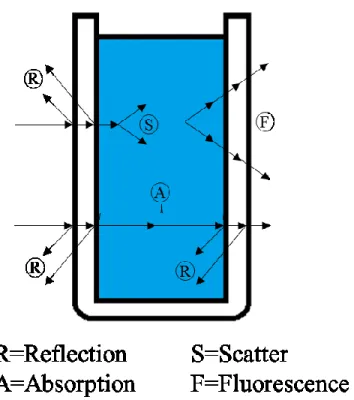
In the environment, the visible light consists of many colors of light. When the light goes through an opaque object, the opaque object absorbs a part of the light. A color of light which is reflected from the object is the color of the object. In the case of the solution, it is the same as the opaque object. The color of the light transmitting solution is the color of the solution [1]. Therefore, each color of the solution absorbs the color of light differently. Furthermore, when the light goes through the solution, the solution does not only absorb one part of the light, it scatters and reflects the light absorbance also shown in figure 2.1. To measure the light absorbance of the solution, the light transmittance is required in calculating. The transmittance (T) is a division between the incident light intensity (𝐼0) and the transmitting light intensity (𝐼) shown in (2.1). The percentage of the transmittance is calculated by (2.2).
𝑇 =𝐼𝐼
0 (2.1)
5
%𝑇 =𝐼𝐼
0× 100 (2.2)
2.1.2. Lambert’s law
Lambert’s law is a method explaining the relation between the light absorbance (A) and the path length (l) that the light transmits a solution. The light absorbance is proportional to the path length for parallel beam and monochromatic radiation transmitting a homogeneous medium with the same concentration in (2.3). There are no unit of the light absorbance.
𝐴 ∝ 𝑙 (2.3)
6
Figure 2.3. Relation between the path length and the transmittance.
Figure 2.4. Relation between the path length and light absorbance.
Figure 2.2 shows the measurement of solution which each solution has the transmittance 50% (%T). It means that when the light goes through solution, the transmitting light intensity remains 50% of the incident light intensity [48]. When the light goes through each medium, the light intensity decreases. It shows that the transmittance is inverse variation with the path length which light goes through. Therefore, the transmission (T) is inverse variation with the path length (l) which the light goes though shown in figure 2.3. The relationship between the transmission (T) and the path length (l) is exhibited in (2.4). 𝑘 is a constant value.
𝑇 =𝐼0
𝐼 = 𝑒−𝑘𝑙 (2.4) To convert the transmittance which is inverse variation with the path length to the light absorbance which is direct variation with the path length, the logarithm is required. Therefore, the determination of the light
0 10 20 30 40 50 60 70 80 90 100 0 2 4 6 8 10 T ran sm ittan ce ( %) Path length (cm) 0 0.5 1 1.5 2 2.5 3 3.5 0 2 4 6 8 10 L ig ht ab so rb an ce ( -) Path length (cm)
7
absorbance is the logarithm of the division between the incident light intensity and the transmitting light intensity in (2.5). The light absorbance value does not have the unit. The relation between the path length and light absorbance shown in figure 2.4. It provides the path length which the light transmits as a medium.
𝐴 = 𝑙𝑜𝑔𝐼0
𝐼 (2.5)
2.1.3. Beer’s law
Beer’s law is a method that explains the relation between the light absorbance and the concentration of solution [1]. The light absorbance (A) is proportional to the concentration of solution (c) for parallel beam and monochromatic radiation transmitting a homogeneous medium with the same path length shown in (2.6). The relationship between the light absorbance and the concentration of solution is illustrated in figure 2.5.
𝐴 ∝ 𝑐 (2.6)
8
Figure 2.6. Relation between the transmittance and concentration.
Figure 2.7. Relation between the light absorbance and concentration.
Figure 2.5 shows that when the concentration of the solution, which the transmittance is 50%, increases to 2 times and 3 times, the light transmittance reduces, respectively. The transmittance is inverse variation with the concentration of solution shown in figure 2.6. The relationship between the light absorbance and the concentration calculated by (2.7) is shown in figure 2.7. 𝑘 is the constant.
𝑇 =𝐼0
𝐼 = 𝑒
−𝑘𝑐 (2.7) To convert the transmittance which is inverse variation with the concentration of solution in figure 2.6 to the light absorbance which is direct variation with the concentration of solution in figure 2.7, the logarithm is necessary. Therefore, the determination of the light absorbance is the logarithm of the division between the
0 10 20 30 40 50 60 70 80 90 100 0 2 4 6 8 10 T ran sm ittan ce ( %)
Concentration of solution (mol/cm2)
0 0.5 1 1.5 2 2.5 3 3.5 0 2 4 6 8 10 L ig ht ab so rb an ce ( -)
9
incident light intensity and the transmitting light intensity in (2.8). It provides the concentration of solution which the light transmits as a medium.
𝐴 = 𝑙𝑜𝑔𝐼0
𝐼 (2.8)
2.1.4. Beer-Lambert’s law
A combination of the two laws defines that a light absorbance (A) is proportional to the path length (l) and the concentration of solution (c) for parallel beam and monochromatic radiation transmitting a homogeneous solution [48]. The transmittance (T) is calculated by (2.9).
𝑇 =𝐼0
𝐼 = 𝑒
−𝑘𝑐𝑙 (2.9) The light absorbance is calculated by taking minus logarithm in (2.9) same as the Beer’s law or Lambert’s law. Therefore, Beer-Lambert’s law equation is shown in (2.10). The molar absorptivity (ɛ) is a coefficient constant value depending on the color of solution and a wavelength of the light source. In some methods, it provides a as the molar absorptivity. In the measurement, the molar absorptivity and the path length of solution are constant. In an experiment, the path length of solution is 1 cm that does not effect for calculation of the concentration. Therefore, it is eliminated.
𝐴 = − log(𝑇) = −log(𝐼𝐼
0) = ɛ𝑐𝑙 (2.10)
From the Beer-Lambert’s law in (2.10), when the concentration (c) is 0 (solvent), the light absorbance (A) is 0. Therefore, in the light absorbance equation (2.10), the incident light intensity (𝐼0) can be changed to the light intensity when the light transmits a solvent (𝐼𝑠𝑜𝑙𝑣𝑒𝑛𝑡). When the solvent is measured, the transmittance is 1. As the result, the light absorbance is 0. Furthermore, the transmitted light intensity (I) is changed to the light transmitting the solution (𝐼𝑠𝑜𝑙𝑣𝑒𝑛𝑡) in (2.11).
𝐴 =
− log
𝐼𝑠𝑜𝑙𝑢𝑡𝑖𝑜𝑛𝐼𝑠𝑜𝑙𝑣𝑒𝑛𝑡 (2.11)
However, there is no the light intensity in the electronic circuit. Therefore, a semiconductor, which converts the light intensity into the electrical value, is used such as LDR (Light dependent resistor), photodiode, phototransistor, etc. The properties of these light detectors depend on the light intensity which they detect. For an example, the phototransistor alters the current flowing according to the light intensity. The increase of the electronic current flowing is logistic growth with the light intensity. A resistance of LDR depends on the light intensity that falls upon itself. The resistance varies inversely with the light intensity. Therefore, the voltage of resistor which is connected with the light detector is inverse variation with the concentration of solution. For this reason, the voltage value (𝑉𝑠𝑜𝑙𝑢𝑡𝑖𝑜𝑛, 𝑉𝑠𝑜𝑙𝑣𝑒𝑛𝑡) can replace the light intensity (𝐼𝑠𝑜𝑙𝑢𝑡𝑖𝑜𝑛, 𝐼𝑠𝑜𝑙𝑣𝑒𝑛𝑡) in (2.12) [56].
𝐴 = − log𝑉𝑠𝑜𝑙𝑢𝑡𝑖𝑜𝑛
𝑉𝑠𝑜𝑙𝑣𝑒𝑛𝑡 (2.12) However, the light absorbance does not vary directly with the concentration of solution in some cases. Therefore, to reduce the number of errors of the measurement, the voltage when there is no light falling on the photo detector (𝑉0) is declined as shown in (2.13) [56].
𝐴 = − log𝑉𝑠𝑜𝑙𝑢𝑡𝑖𝑜𝑛−𝑉0
10
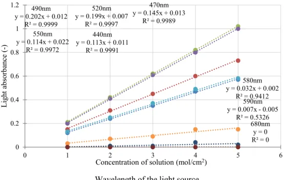
Figure 2.8. Light absorbance of red solution by many wavelengths of the light source.
From the Beer-Lambert’s law in (2.10), the light absorbance depends on the molar absorptivity (ɛ), the concentration of solution (𝑐) and the path length of the light (𝑙). In the measurement, the path length is constant value and the concentration is unknown value. Therefore, the light absorbance value depends on the molar absorptivity. Figure 2.8 shows the light absorbance results of the red solution in many cases of the wavelength of the light source by Biochrom WPA CO7500 Colorimeter. The alteration of the wavelength of a light source changes the molar absorptivity. There are many cases which can observe the rising of the light absorbance or cannot observe. To calculate the concentration of solution easily and observe the growth light absorbance simply, the case of the highest light absorbance (the highest molar absorptivity) is provided to make the linear regression equation.
2.1.5. Coefficient of determination
Although the concentration calculation by the highest molar absorptivity is the best, it does not mean that the light absorbance of other wavelengths cannot be used to calculate the concentration of solution. The coefficient of determination is a value that indicates how well data fit with a statistic model. In the light absorbance measurement, it is used to check how well of the relationship between the light absorbance and the concentration of solution as Beer-Lambert’s law. The coefficient of determination is calculated by the square of the correlation coefficient (R2) in (2.14) [57-58]. x is the concentration of solution and y is the light absorbance. 𝑥̅ is an average of the concentration of solution and 𝑦̅ is an average of the light absorbance. N is the number of the data (the number of the known concentration solutions).
𝑅
2= {
∑𝑁𝑖=1(𝑥𝑖−𝑥̅)(𝑦𝑖−𝑦̅) √∑𝑁𝑖=1(𝑥𝑖−𝑥̅)2∑𝑁𝑖=1(𝑦𝑖−𝑦̅)2}
2 (2.14) 440nm y = 0.113x + 0.011 R² = 0.9991 470nm y = 0.145x + 0.013 R² = 0.9989 490nm y = 0.202x + 0.012 R² = 0.9999 520nm y = 0.199x + 0.007 R² = 0.9997 550nm y = 0.114x + 0.022 R² = 0.9972 580nm y = 0.032x + 0.002 R² = 0.9412 590nm y = 0.007x - 0.005 R² = 0.5326 680nm y = 0 R² = 0 0 0.2 0.4 0.6 0.8 1 1.2 0 1 2 3 4 5 6 L ig ht ab so rb an ce ( -)Concentration of solution (mol/cm2)
440nm 470nm 490nm 520nm 550nm 580nm 590nm 680nm
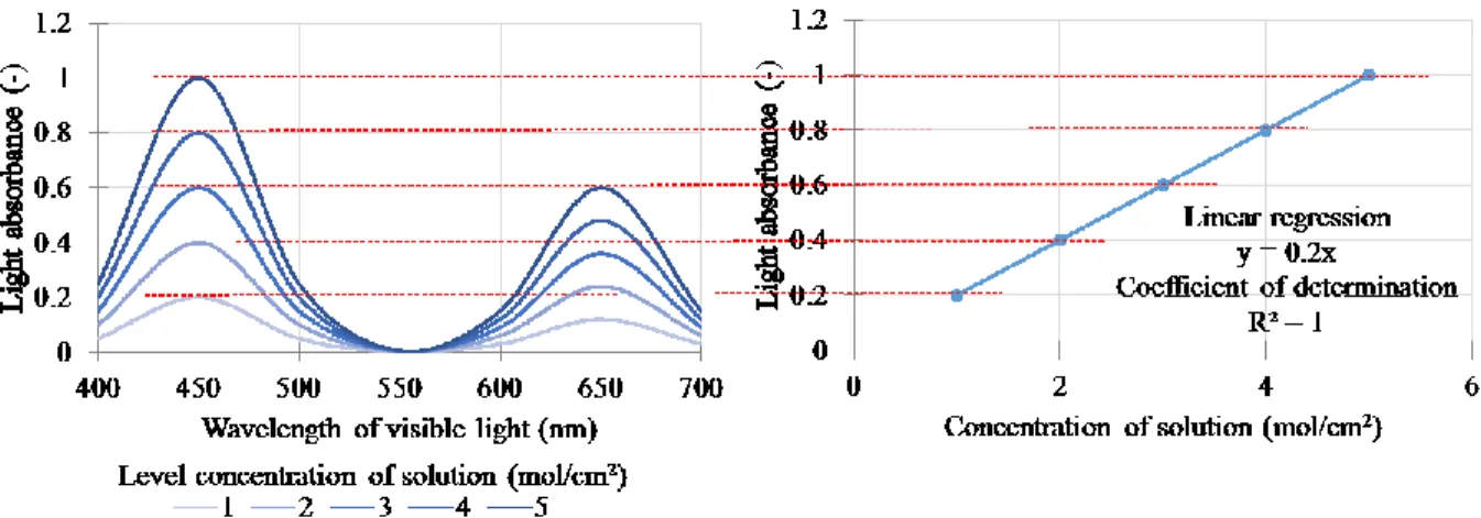
11
A range of the coefficient of determination is from 0 to 1. An ideal value is 1 when y varied directly with x perfectly shown in figure 2.9. It means that if the coefficient of determination is approximate to 1, the
relation between the light absorbance and the concentration of solution is followed in Beer-Lambert’s law. To calculate the concentration of solution efficiently, the wavelength that the coefficient of determination is approximate to 1 is utilized.
2.1.6. Linear regression analysis
To calculate the concentration of solution from the light absorbance, a spectrophotometric method is used. In a pure solution case, the spectrophotometric method provides a linear regression analysis. The linear regression analysis provides many known concentration solutions to calculate a linear function that is a relationship between the light absorbance and concentration following Beer-Lambert’s law shown in figure 2.9. The linear function is shown in (2.15) [59].
Y=a+bX
(2.15) When the linear regression equation in (2.15) is compared with the Beer-Lambert’s law in (2.10), Y is the light absorbance (𝐴). X is the concentration of solution (𝑐). b is the molar absorptivity (ɛ) and the path length (𝑙) which is a constant value. a is the light absorbance when the concentration is 0. In an ideal term, a is 0 following Beer’s laws equation in (2.10). However, in the measurement, there are some errors. Therefore, a is almost zero. b is a slope of the graph which is calculated by (2.16). a is the light absorbance when the concentration is 0. It is calculated by (2.17). N is the number of the data (the number of the known concentration solutions).𝑏 =
∑ 𝑋𝑖𝑌𝑖− ∑𝑁𝑖=0𝑋𝑖∑𝑁𝑖=0𝑌𝑖 𝑁 𝑁 𝑖=0 (∑𝑁𝑖=0𝑋𝑛2)−𝑁(𝑋̅)2 (2.16)𝑎 = 𝑌̅ − 𝑏𝑋̅
(2.17)Figure 2.9. Ideal light absorbance.
Linear regression y = x Coefficient of determination R² = 1 0 1 2 3 4 5 6 7 0 1 2 3 4 5 6 7 L ig ht ab so rb nac e (-)
12
Figure 2.10. Design of linear function that is the relation between the concentration and the light absorbance. To calculate the concentration of the solution, the light absorbance of the solution is measured by a spectrophotometer. The left-hand graph of figure 2.10 illustrates examples of the light absorbance in the range of the visible spectrum wavelength about 380-740 nm. The spectrophotometer provides the light in the visible spectrum wavelength as a light source to measure the light absorbance. To calculate the concentration clearly, the linear regression analysis provides the light absorbance of many concentrations to calculate the linear function in the right-hand graph of figure 2.10. The light absorbance is provided is the highest light absorbance in the range of the visible light at 450 nm of wavelength. The linear function is the relation between the concentration of solution and the light absorbance in (2.15). Therefore, when the light absorbance is measured, the concentration is calculated by the linear function calculated by the linear regression analysis in the case of the pure solution [1,48].
2.1.7. Multicomponent
However, in the case of the multi-component solution, the light absorbance of the mixture solution (
𝐴
𝑀)
is the sum of the light absorbances of each component shown in (2.18). Therefore, the concentration of the components cannot be calculated by the linear regression analysis directly. To analyze the concentration of the components, there must be use of any methods shown in section 2.2.
13
2.2. Comparison of the multicomponent analysis
In this section, the explanation about the previous multi-component spectrophotometric techniques is presented. There are the calculation, advantages, and disadvantages of each method. Each technique has a different calculation process. After that, they are compared by the number of the inputs, the linear regression calculation time and the specific condition.
2.2.1. Simultaneous equation method
The simultaneous equation method is a simple mathematic to calculate the concentration of solution [17-22]. This technique requires the number of the light absorbance equation in any wavelengths equal to the number of the components in the mixture solution. In the case of the 2 components, the light absorbance is the sum of the light absorbance of 2 components. The light absorbance (𝐴𝑀1, 𝐴𝑀2) is measured by wavelength 1 and wavelength 2 shown in (2.19) and (2.20), respectively. The components in the mixture consist of the substance x and substance y. 𝑐𝑥 and 𝑐𝑦 are the concentration of solution of substance x and substance y, respectively. 𝑎𝑥1 and 𝑎𝑥2 are the molar absorptivity between the substance x and wavelength 1 and wavelength
2, respectively. 𝑎𝑦1 and 𝑎𝑦2 are the molar absorptivity between the substance y and wavelength 1 and wavelength 2, respectively.
𝐴
𝑀1= 𝑎
𝑥1𝑐
𝑥+ 𝑎
𝑦1𝑐
𝑦(2.19)
𝐴
𝑀2= 𝑎
𝑥2𝑐
𝑥+ 𝑎
𝑦2𝑐
𝑦(2.20)
To calculate the concentration of each component, the equations (2.19) and (2.20) are rewritten by (2.21) and (2.22), respectively.
𝑐
𝑥=
𝐴𝑀2−𝑎𝑦2𝑐𝑦𝑎𝑥2
(2.21)
𝑐
𝑦=
𝐴𝑀1𝑎−𝑎𝑥1𝑐𝑥𝑦1
(2.22)
The simultaneous equation technique eliminates the disinterest component variable from the light absorbance equation by substituting. The concentration of the substance x (𝑐𝑥) in (2.21) are substituted into (2.20). The concentration of the substance y (𝑐𝑦) in (2.22) is substituted into (2.19). The rewritten equation is obtained in (2.23) and (2.24) that are the concentration of the substance x and substance y, respectively.
𝑐
𝑥=
𝑎𝑦1𝐴𝑀2−𝑎𝑦2𝐴𝑀1𝑎𝑥2𝑎𝑦1−𝑎𝑦2𝑎𝑥1
(2.23)
𝑐
𝑦=
𝑎𝑎𝑥2𝐴𝑀1−𝑎𝑥1𝐴𝑀2𝑥2𝑎𝑦1−𝑎𝑦2𝑎𝑥1
(2.24)
The process of the simultaneous equation method is shown in figure 2.11. To calculate the concentration, the molar absorptivity is calculated by the slope of the linear regression equation. It is calculated by the known concentration data in (2.16). X is the concentration of the component and Y is the light absorbance of pure solution. After that, the concentration calculation provides the light absorbance measured by 2 wavelengths and the molar absorptivity calculated by the linear regression analysis in (2.23) and (2.24).
14
Figure 2.11. Process of the simultaneous equation method.
2.2.2.
Derivative spectrophotometry
This method relates to the alternation of the absorption spectra or the zero-order spectrum to the first-order derivative spectrum or the high first-order [23-28,60]. The width of the high-first-order wave is narrower than the width of the low-order wave. Therefore, the high order spectrum has more detail than the low order spectrum. Figure 2.12 illustrates examples of the light absorbance of the component x, component y, and mixture between component x and y that the spectrum is overlapped by the light absorbance of component x and component y. The light absorbance of the mixture is calculated by (2.25). ɛ𝑥 and ɛ𝑦 are the molar absorptivity of component
x and component y.
𝐴
𝑀= ɛ
𝑥𝑐
𝑥𝑙 + ɛ
𝑦𝑐
𝑦𝑙 (2.25)
Figure 2.12. Example light absorbance. 0 0.2 0.4 0.6 0.8 1 1.2 1.4 1.6 350 400 450 500 550 600 650 700 L ight abs or bance (-)
Wavelength of visible light (nm)
x y x+y
Light absorbance of component x (𝐴𝑥) Light absorbance of component y (𝐴𝑦) Light absorbance of mixture (𝐴𝑀) Known concentration data of pure
solution at each wavelength
Linear
regression
analysis
Molar absorptivity
(𝑎
𝑥1, 𝑎
𝑦1, 𝑎
𝑥2, 𝑎
𝑦2)
Concentration of the
component x (𝑐
𝑥) and
component y (𝑐
𝑦)
Concentration
calculation
equation
Light absorbance of the
wavelength 1 (𝐴
𝑀1) and
15
The derivative first order of the light absorbance by wavelength is presented in (2.26). In the derivative of light absorbance by wavelength, the concentration of the component and the path length are a constant value. The alteration is only the molar absorptivity.
𝑑𝐴𝑀 𝑑𝜆
= 𝑐
𝑥𝑙
𝑑ɛ𝑥 𝑑𝜆+ 𝑐
𝑦𝑙
𝑑ɛ𝑦 𝑑𝜆(2.26)
Figure 2.13 displays the derivative first order of the light absorbance of figure 2.12. It shows that at the wavelength which the light absorbance is the peak of wave, the pure component amplitude of the first order derivative is 0. This point is called “zero-crossing”. Therefore, the derivative spectrophotometer method provides the zero-crossing point to eliminate the disinterest component variable. The amplitude of the first-order at the zero-crossing which the light absorbance of the substance y is maximum is obtained in (2.27).
𝑑𝐴𝑀
𝑑𝜆
= 𝑐
𝑥𝑙
𝑑ɛ𝑥𝑑𝜆
(2.27)
The amplitude of the first order in (2.27) shows that the variable of the component y is obliterated and the concentration of the component x (𝑐𝑥) is direct variation with the mixture amplitude of the first order (𝑑𝐴𝑑𝜆𝑀). Figure 2.14 illustrates the relationship of the first derivative of the mixture light absorbance when the concentration of component y increases. It shows that the amplitude of the first derivative at the zero-crossing when the light absorbance of component y is at the peak of the wave in zero-order is equal in every solution even if the concentration of the component y is changed. Furthermore, figure 2.15 illustrates the amplitude of the first derivative at the zero-crossing when the light absorbance of component x is at the peak of the curve in zero order. The amplitude of the first derivative is direct variation with the concentration of the component y.
Figure 2.13. First order derivative of example light absorbance. -0.02 -0.015 -0.01 -0.005 0 0.005 0.01 0.015 0.02 350 400 450 500 550 600 650 700 dA /d λ (-)
Wavelengtht of visible light (nm)
x y x+y
zero-crossing
zero-crossing
Derivative 1storder of light absorbance of component x (𝑑𝐴𝑥
𝑑λ)
Derivative 1storder of light absorbance of component y (𝑑𝐴𝑦
𝑑λ)
Derivative 1storder of light absorbance of mixture (𝑑𝐴𝑀
16
Figure 2.14. First order derivative light absorbance of the mixture solution when the concentration of component y increase.
Figure 2.15. Amplitude of the first derivative at the zero-crossing when the light absorbance of component x is peak of the curve in zero order.
-0.03 -0.025 -0.02 -0.015 -0.01 -0.005 0 0.005 0.01 0.015 0.02 0.025 350 400 450 500 550 600 650 700 dA /d λ
Wavelength of visible light (nm)
x+y
x+2y
x+3y
Zero-crossing wavelength when the light absorbance of component y is the peak of curve in zero order.
Zero-crossing wavelength when the light absorbance of component x is the peak of curve in zero order.
Derivative 1storder of light absorbance of mixture when the concentration of the component y is level 1 (𝑑(𝐴𝑑𝑥λ+𝐴𝑦))
Derivative 1storder of light absorbance of mixture when the concentration of the component y is level 2 (𝑑(𝐴𝑥𝑑+2𝐴λ 𝑦))
Derivative 1storder of light absorbance of mixture when the concentration of the component y is level 3 (𝑑(𝐴𝑥𝑑+3𝐴λ 𝑦)) y = 0.0073x R² = 1 0 0.005 0.01 0.015 0.02 0.025 0 0.5 1 1.5 2 2.5 3 3.5 dA /d λ
17
Figure 2.16. Process of the derivative method.
Process of the derivative spectrophotometry is displayed in figure 2.16. The light absorbance at the zero crossing is taken by derivative to eliminate the noise of the disinterest component. Therefore, the derivative first order amplitude of the light absorbance of the mixture is direct variation with the concentration of the interest component at the zero-crossing. The linear regression analysis calculates the linear function that is the relation between the first order amplitude and the concentration of the known concentration solution to calculate the concentration of solution.
2.2.3.
Absorb ratio method
This method utilizes the division by the standard solution of the disinterest solution [29-31]. To eliminate the variable of the disinterest solution, the light absorbance ratio between the mixture and the disinterest standard solution is subtracted by the light absorbance ratio between the mixture and the disinterest standard solution of another wavelength. The light absorbance of the mixture solution (𝐴𝑀) between component x and component y is the sum of the light absorbance of component x (𝐴𝑥) and y (𝐴𝑦) in (2.28).
𝐴M= 𝐴𝑥+ 𝐴𝑦 (2.28) The ratio between light absorbance of the mixture solution between component x and component y (𝐴𝑀) and the standard solution (𝐴0𝑥) of x substance is presented in (2.29).
𝐴𝑀 𝐴𝑥0 = 𝐴𝑥 𝐴𝑥0
+
𝐴𝑦 𝐴𝑥0 (2.29) Figure 2.17 shows examples of the light absorbances of component x, component y and the mixture between component x and component y. The light absorbance ratio between the standard of the component x and mixture solutions is shown in figure 2.18. It shows that the light absorbance ratio between the disinterest component and the standard solution (𝐴𝑥𝐴𝑥0
)
is constant in every wavelength. Therefore, the difference between the mixture ratio (𝐴𝑀𝐴𝑥0) and the component y ratio ( 𝐴𝑦
𝐴𝑥0) is equal in every wavelength. The equation (2.30) is the light absorbance ratio between the mixture and the standard solution of the wavelength 1 is subtracted by the light absorbance ratio between the mixture and the standard solution in wavelength 2.
[𝐴𝑀 𝐴𝑥0] 1− [ 𝐴𝑀 𝐴𝑥0] 2= [ 𝐴𝑦 𝐴𝑥0] 1− [ 𝐴𝑦 𝐴𝑥0] 2 (2.30) When the concentration of the component y is factorized from the light absorbance, the equation (2.31) is obtained.
Derivative 1st order Linear regression analysis
Known concentration light absorbances at the zero
crossing Light absorbance at
the zero crossing
Concentration of the component x (𝑐𝑥) and component y (𝑐𝑦) Derivative 1st order
18 {[𝜀𝑦 𝐴𝑥0] 1− [ 𝜀𝑦 𝐴𝑥0] 2} 𝑐𝑦= [ 𝐴𝑀 𝐴𝑥0] 1− [ 𝐴𝑀 𝐴𝑥0] 2 ( 2 . 3 1 )
Figure 2.17. Example light absorbance for the absorb ratio method.
Figure 2.18. Ratio between the light absorbance of component x, component y and mixture and standard of component x. 0 0.2 0.4 0.6 0.8 1 1.2 1.4 1.6 400 450 500 550 600 650 700 L ight abs or bance
Wavelength of visible light (nm)
x y x+y
Light absorbance of component x (𝐴𝑥) Light absorbance of component y (𝐴𝑦) Light absorbance of mixture (𝐴𝑀)
0 1 2 3 4 5 6 7 8 400 450 500 550 600 650 700 A m plitu de (-)
Wavelength of visible light (nm)
x/x0 y/x0 (x+y)/x0 𝐴𝑦 𝐴𝑥0 1− 𝐴𝑦 𝐴𝑥0 2 𝐴𝑀 𝐴𝑥0 1 − 𝐴𝑀 𝐴𝑥0 2
Light absorbance ration between component x and standard of component x (𝐴𝑥
𝐴𝑥0)
Light absorbance ration between component y and standard of component x (𝐴𝐴𝑦
𝑥 0)
Light absorbance ration between mixture and standard of component x (𝐴𝑀
19
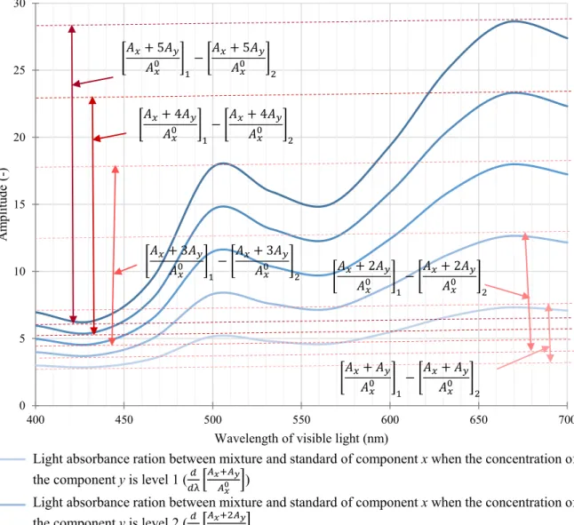
Figure 2.19. Light absorbance ratio between the mixture solution and standard solution of component x when concentration of the component y increases.
0 5 10 15 20 25 30 400 450 500 550 600 650 700 A m plitu de (-)
Wavelength of visible light (nm)
(x+y)/x0 (x+2y)/x0 (x+3y)/x0 (x+4y)/x0 (x+5y)/x0 𝐴𝑥+ 5𝐴𝑦 𝐴𝑥0 1− 𝐴𝑥+ 5𝐴𝑦 𝐴𝑥0 2 𝐴𝑥+ 4𝐴𝑦 𝐴𝑥0 1− 𝐴𝑥+ 4𝐴𝑦 𝐴𝑥0 2 𝐴𝑥+ 3𝐴𝑦 𝐴0𝑥 1− 𝐴𝑥+ 3𝐴𝑦 𝐴𝑥0 2 𝐴𝑥+ 2𝐴𝑦 𝐴𝑥0 1− 𝐴𝑥+ 2𝐴𝑦 𝐴𝑥0 2 𝐴𝑥+ 𝐴𝑦 𝐴𝑥0 1− 𝐴𝑥+ 𝐴𝑦 𝐴𝑥0 2
Light absorbance ration between mixture and standard of component x when the concentration of the component y is level 1 (𝑑
𝑑λ 𝐴𝑥+𝐴𝑦
𝐴𝑥0 )
Light absorbance ration between mixture and standard of component x when the concentration of the component y is level 2 (𝑑λ𝑑 𝐴𝑥+2𝐴𝐴 𝑦
𝑥 0
Light absorbance ration between mixture and standard of component x when the concentration of the component y is level 3 (𝑑λ𝑑 𝐴𝑥+3𝐴𝐴 𝑦
𝑥 0 )
Light absorbance ration between mixture and standard of component x when the concentration of the component y is level 4 (𝑑λ𝑑 𝐴𝑥+4𝐴𝐴 𝑦
𝑥 0 )
Light absorbance ration between mixture and standard of component x when the concentration of the component y is level 5 (𝑑
𝑑λ
𝐴𝑥+5𝐴𝑦
20
Figure 2.20. Difference of the light absorbance ratio (𝐴𝑥+𝐴𝑦
𝐴𝑥0 ) between wavelength 1 and wavelength 2 when
the concentration of component y increases.
Figure 2.21. Process of the absorbance ratio method. {[𝜀𝑦
𝐴𝑥0]
1− [ 𝜀𝑦
𝐴𝑥0]
2} is constant. Therefore, the concentration of component y (𝑐𝑦) is proportional to the different of the light absorbance ratio between mixture solution and standard of the disinterest component of both wavelengths ([𝐴𝑀
𝐴𝑥0]
1− [ 𝐴𝑀 𝐴𝑥0]
2). Figure 2.19 shows the light absorbance ratio between the mixture solution and the disinterest standard solution of both wavelengths. It demonstrates that when the concentration of the component y increases, the difference of the light absorbance ratio (𝐴𝑀
𝐴𝑥0) between wavelength 1 and wavelength 2 increases also. The difference of the light absorbance ratio (𝐴𝑀
𝐴𝑥0) between wavelength 1 and wavelength 2
([𝐴𝑀
𝐴𝑥0]1− [ 𝐴𝑀
𝐴𝑥0]2) varies with the concentration of the component y (𝑐𝑦) directly shown on figure 2.20. The concentration of the component y can be calculated by linear regression analysis.
Process of the absorbance ratio method is exhibited in figure 2.21. The difference of the light absorbance between 2 wavelengths is divided by the disinterest standard solution to eliminate the disinterest component.
y = 4.4532x R² = 1 0 5 10 15 20 25 0 1 2 3 4 5 6 Dif fer en ce am plitu de (-)
Concentration of component y (mol/cm2)
Difference light absorbance between wavelength 1 and
wavelength 2 (𝐴1− 𝐴2)
Division by light absorbance of standard solution (𝐴𝑥0, 𝐴𝑦0)
Linear regression analysis
Difference light absorbance of the known concentrations between wavelength 1 and wavelength 2
Concentration of the component x (𝑐𝑥) and
component y (cy) Division by standard solution (𝐴𝑥0, 𝐴0𝑦)
21
Therefore, there is no noise of the disinterest component in the difference of the light absorbance ratio. The difference of the light absorbance ratio varies the concentration of interest component directly. Thus, the linear regression analysis calculates the linear function that is the relation between the difference of the light absorbance ratio and the concentration of the known concentration solution to calculate the concentration of solution.
2.2.4.
Derivative ratio spectra method
The derivative ratio spectra method is based on the derivative spectra and the absorbance ratio method [32-36]. This technique continues from (2.29). The derivative first-order of (2.29) by wavelength is obtained in (2.32). 𝑑 𝑑𝜆[ 𝐴𝑀 𝐴0𝑥] = 𝑑 𝑑𝜆[ 𝐴𝑥 𝐴𝑥0+ 𝐴𝑦 𝐴𝑥0] (2.32) The light absorbance ratio between component x and the standard of component x (𝐴𝑥
𝐴𝑥0) is constant.
Therefore, it is eliminated. The derivative of the light absorbance ratio is shown in (2.33). 𝑑 𝑑𝜆[ 𝐴𝑀 𝐴0𝑥] = 𝑑 𝑑𝜆[ 𝐴𝑦 𝐴𝑥0] (2.33)
Figure 2.22 shows the derivative of the light absorbance ratio from figure 2.18. It presents that the derivative of the light absorbance ratio between mixture solution and the standard of the component x (𝑑𝜆𝑑 [𝐴𝑀
𝐴𝑥0])
is equal to the light absorbance ratio between component y and the standard of the component x (𝑑𝜆𝑑 [𝐴𝑦
𝐴𝑥0]). The
concentration (𝑐𝑦) and the path length (l) are factors of the light absorbance which do not alter by the wavelength in (2.34). Therefore, they can be factorized from the light absorbance, the equation (2.35) is obtained.
𝐴𝑦= 𝑐𝑦𝑙𝜀𝑦 ( 2 . 3 4 ) 𝑑 𝑑𝜆[ 𝐴𝑀 𝐴0𝑥] = 𝑐𝑦𝑙𝑑𝜆𝑑 [ 𝜀𝑦 𝐴𝑥0] (2.35)
It shows that the concentration of the component y (𝑐𝑦) is direct variation with the derivative of the light absorbance ratio between mixture solution and the standard of the component x (𝑑𝜆𝑑 [𝐴𝑀
𝐴𝑥0]) in every
22
Figure 2.22. Derivative of the ratio of the light absorbance from Figure 2.18.
Figure 2.23. Process of the derivative ratio method.
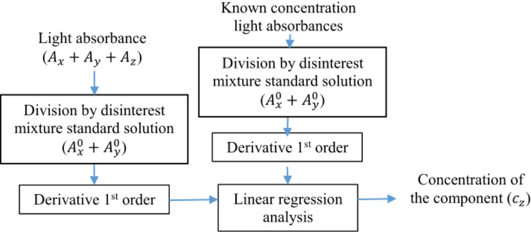
Process of the derivative ratio method is exhibited in figure 2.23. The light absorbance is divided by the disinterest standard solution. After that, to eliminate the disinterest component, the light absorbance ratio is differentiated. The derivative light absorbance ratio does not have the noise of the disinterest component. Therefore, it varies the concentration of solution directly. Thus, the linear regression analysis calculates the linear function that is the relation between the derivative light absorbance ratio and the concentration of the known concentration solution to calculate the concentration of solution.
-5 0 5 10 15 20 25 30 35 400 450 500 550 600 650 700 d( A m pli tu te)/d λ
Wavelength of the visible light (nm)
d(x/x0)/dλ
d(y/x0)/dλ
d(x+y/x0)/dλ
Derivative 1storder of the light absorbance ratio between component x and standard of component x (𝑑λ𝑑 𝐴𝐴𝑥
𝑥 0 )
Derivative 1storder of the light absorbance ratio between component y and standard of component x (𝑑λ𝑑 𝐴𝐴𝑦
𝑥 0 )
Derivative 1storder of the light absorbance ratio between mixture and standard of component x (𝑑λ𝑑 𝐴𝑀 𝐴𝑥0 ) 𝑑 𝑑λ 𝐴𝑥 𝐴𝑥0 𝑑 𝑑λ 𝐴𝑦 𝐴𝑥0 𝑑 𝑑λ 𝐴𝑀 𝐴𝑥0
Derivative 1st order Linear regression analysis Known concentration light
absorbances Concentration of the component x (𝑐𝑥) and component y (𝑐𝑦) Division by standard solution (𝐴𝑥0, 𝐴𝑦0) Light absorbance Derivative 1st order Division by standard solution
23
2.2.5. Double divisor ratio spectra derivative method
This method is based on the derivative ratio spectra method [49-50]. It analyses the 3 compounds of the mixture solution. The light absorbance of 3 compounds mixture solution is shown in (2.36). The mixture consists of component x, component y, and component z.
𝐴𝑀= 𝑎𝑥𝑐𝑥+ 𝑎𝑦𝑐𝑦+ 𝑎𝑧𝑐𝑧 (2.36) It is the same as the absorbance ratio method that provides the standard of disinterest solution. In this method, there are 3 compounds in the mixture. Therefore, the standard solution is the mixture solution of 2 disinterest compounds shown in (2.37).
𝐴𝑀0 = 𝑎𝑥𝑐𝑥0+ 𝑎𝑦𝑐𝑦0 (2.37) The ratio between the mixture solution of 3 compounds and the standard mixture of 2 of 3 compounds of the mixture solution (𝐴𝑀
𝐴𝑀0) is obtained in (2.38). 𝐴𝑀 𝐴𝑀0 = 𝑎𝑥𝑐𝑥+𝑎𝑦𝑐𝑦 𝑎𝑥𝑐𝑥0+𝑎𝑦𝑐𝑦0+ 𝑎𝑧𝑐𝑧 𝑎𝑥𝑐𝑥0+𝑎𝑦𝑐𝑦0 (2.38)
The first derivative of the mixture solution of 3 compounds and the standard mixture of 2 of 3 compounds of the mixture solution (𝐴𝑀
𝐴𝑀0) is shown in (2.39). 𝑑 𝑑𝜆[ 𝐴𝑀 𝐴𝑀0] = 𝑑 𝑑𝜆[ 𝑎𝑥𝑐𝑥+𝑎𝑦𝑐𝑦 𝑎𝑥𝑐𝑥0+𝑎 𝑦𝑐𝑦0] + 𝑑 𝑑𝜆[ 𝑎𝑧𝑐𝑧 𝑎𝑥𝑐𝑥0+𝑎 𝑦𝑐𝑦0] (2.39)
The light absorbance ratio between the 2 compounds which is the mixture and the standard mixture (𝑎𝑥𝑐𝑥+𝑎𝑦𝑐𝑦
𝑎𝑥𝑐𝑥0+𝑎
𝑦𝑐𝑦0) is as constant as to the ratio of disinterest component (
𝐴𝑥
𝐴𝑥0) in (2.32) in the case of the concentration
ratio (𝑐𝑥
𝑐𝑦) between the component x and component y is equal with the concentration ration of the standard mixture (𝑐𝑥0
𝑐𝑦0) between component x and component y. Therefore, the equation (2.40) is obtained.
𝑑 𝑑𝜆[ 𝐴𝑀 𝐴𝑀0] = 𝑑 𝑑𝜆[ 𝑎𝑧𝑐𝑧 𝑎𝑥𝑐𝑥0+𝑎 𝑦𝑐𝑦0] (2.40)
It presents that the concentration of the interest component (𝑐𝑧) is direct variation with the derivative first order of the light absorbance ratio between the mixture solution (𝐴𝑀) and the standard mixture solution (𝐴𝑀0). Thus, the concentration of the component z can be calculated by linear regression analysis with the derivative of the light absorbance ratio (𝑑𝜆𝑑 [𝐴𝑀
𝐴𝑀0]) between the mixture solution and the standard of mixture
solution. However, in the case that the ratio of the disinterest component is not equal to the ratio of the disinterest standard component, the equation (2.41) is obtained.
𝑑 𝑑𝜆[ 𝐴𝑀 𝐴𝑀0] − 𝑑 𝑑𝜆[ 𝑎𝑥𝑐𝑥+𝑎𝑦𝑐𝑦 𝑎𝑥𝑐𝑥0+𝑎𝑦𝑐𝑦0] = 𝑑 𝑑𝜆[ 𝑎𝑧𝑐𝑧 𝑎𝑥𝑐𝑥0+𝑎𝑦𝑐𝑦0] (2.41)
Figure 2.24 displays the light absorbance of the 3 components and the mixture solution of 3 components. Figure 2.25 exhibits the derivative ratio of the light absorbance in figure 2.24. It shows that when the concentration ratio of disinterest component (𝑐𝑥
𝑐𝑦) is not equal to the concentration ratio of disinterest standard component (𝑐𝑥0
24
mixture (𝑑𝜆𝑑 [𝐴𝑥+2𝐴𝑦
𝐴𝑥0+𝐴 𝑦
0]) is not 0. However, when the light absorbance ratio of mixture (
𝑑 𝑑𝜆[ 𝐴𝑥+2𝐴𝑦+𝐴𝑧 𝐴𝑥0+𝐴 𝑦 0 ]) is
substituted by the light absorbance ratio of the disinterest solution (𝑑𝜆𝑑 [𝐴𝑥+2𝐴𝑦
𝐴𝑥0+𝐴 𝑦
0]), the result is equal to the light
absorbance ratio of mixture (𝑑𝜆𝑑 [𝐴𝑥+𝐴𝑦+𝐴𝑧
𝐴0𝑥+𝐴 𝑦
0 ]) in case of the ratio of the component is equal to the ratio of the
standard component.
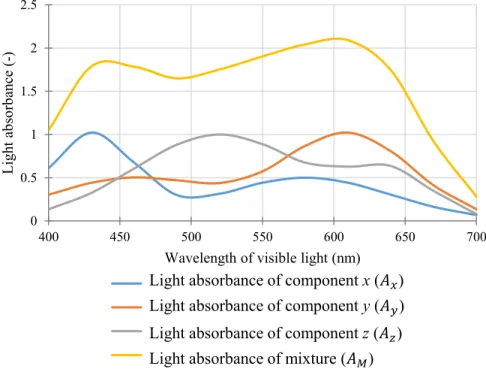
Figure 2.24. Light absorbance of 3 components and the mixture solution of 3 components. 0 0.5 1 1.5 2 2.5 400 450 500 550 600 650 700 L ig ht ab so rb ance (-)
Wavelength of visible light (nm)
x y z x+y+z
Light absorbance of component x (𝐴𝑥)
Light absorbance of component y (𝐴𝑦) Light absorbance of component z (𝐴𝑧) Light absorbance of mixture (𝐴𝑀)