JAIST Repository: Counterexample-guided abstraction refinement for points-to analysis of object-oriented programs

全文

(1)JAIST Repository https://dspace.jaist.ac.jp/. Title. Counterexample-guided abstraction refinement for points-to analysis of object-oriented programs. Author(s). Vu, Quang Vinh. Citation Issue Date. 2016-09. Type. Thesis or Dissertation. Text version. author. URL. http://hdl.handle.net/10119/13740. Rights Description. Supervisor:寺内多智弘, 情報科学研究科, 修士. Japan Advanced Institute of Science and Technology.

(2) Counterexample-guided abstraction refinement for points-to analysis of object-oriented programs. Vu Quang Vinh School of Information Science Japan Advanced Institute of Science and Technology September, 2016.

(3) Master’s Thesis. Counterexample-guided abstraction refinement for points-to analysis of object-oriented programs. 1410213 Vu Quang Vinh. Supervisor : Professor Tachio Terauchi Main Examiner : Professor Tachio Terauchi Examiners : Professor Mizuhito Ogawa Associate professor Nao Hirokawa. School of Information Science Japan Advanced Institute of Science and Technology August, 2016.

(4) Acknowledgement First and foremost, I would like to express my sincere gratitude to my advisor Prof. Tachio Terauchi of the School of Information Science at Japan Advanced Institute of Science and Technology for his kindly carefully guidance and supports. I greatly appreciate his expertise, understanding, patience, and tolerating my mistakes. A very special thanks goes out to Prof. Mizuhito Ogawa and Assoc. Prof. Nao Hirokawa. They provided me with directions and constructive comments. I wish to say thank you to all members of Terauchi-laboratory of the Information Science School at JAIST for helping me to adapt to the new living condition in Japan. I recognize that this research would not have been possible without the financial aid of the JAIST-scholarship for the joint program with Vietnam National University, Ho Chi Minh City (VNU-HCM). I also would like to thank the scholarship from the Japan Student Services Organization (JASSO) for supporting me the living expenses for 6-month study in Japan. Finally, from the bottom of my heart, I want to express my gratitude to my parents and my sister for their continuous encouragement through the process of my research, writing this thesis and also my years of studying. This accomplishment would not have achieved without them.. i.

(5) Contents 1 Introduction 1.1 Points-to analysis . . . . 1.2 Problem . . . . . . . . . 1.3 Method and experiments 1.4 Contributions . . . . . . 1.5 Outline for later chapters. . . . . .. . . . . .. . . . . .. . . . . .. . . . . .. . . . . .. . . . . .. . . . . .. . . . . .. . . . . .. . . . . .. 1 1 2 3 4 4. . . . . . . . . . . . . . . . . . . sensitivity . . . . . . . . . . . . . . . . . .. . . . . . . .. . . . . . . .. . . . . . . .. . . . . . . .. . . . . . . .. . . . . . . .. . . . . . . .. . . . . . . .. . . . . . . .. . . . . . . .. 5 5 6 9 12 12 12 14. 3 Proposed method 3.1 Adaptive points-to analysis . . . . . . . . . . . . . . . . . . . . . . . . . 3.2 Problem restatement . . . . . . . . . . . . . . . . . . . . . . . . . . . . 3.3 CEGAR-based algorithm . . . . . . . . . . . . . . . . . . . . . . . . . . 3.3.1 Choosing abstraction with by maximum satisfiability (MaxSAT) 3.4 Provenances vs Datalog runs . . . . . . . . . . . . . . . . . . . . . . . . 3.5 Cheap abstraction for refinement . . . . . . . . . . . . . . . . . . . . . 3.6 Partitioned abstraction search . . . . . . . . . . . . . . . . . . . . . . . 3.7 Repeated abstraction search . . . . . . . . . . . . . . . . . . . . . . . .. . . . . . . . .. . . . . . . . .. 15 15 17 17 19 20 21 21 22. . . . . .. . . . . .. . . . . .. . . . . .. . . . . .. . . . . .. . . . . .. . . . . .. . . . . .. . . . . .. . . . . .. . . . . .. 2 Background 2.1 Static analysis in Datalog . . . . . . . . . . . 2.2 Simple points-to analysis program . . . . . . . 2.3 Context-sensitive points-to analysis . . . . . . 2.4 Call-site sensitivity, object sensitivity and type 2.4.1 Call-site sensitivity . . . . . . . . . . . 2.4.2 Object sensitivity and type sensitivity 2.5 Abstraction . . . . . . . . . . . . . . . . . . .. . . . . .. . . . . .. . . . . .. . . . . .. . . . . .. 4 Related works 24 4.1 Pushdown system . . . . . . . . . . . . . . . . . . . . . . . . . . . . . . . . 24 4.2 Abstraction Refinement . . . . . . . . . . . . . . . . . . . . . . . . . . . . 25 5 Implementation 26 5.1 Eliminate non-context predicates from counterexample knowledge . . . . . 26 5.2 Trace tuples from may fail downcasts . . . . . . . . . . . . . . . . . . . . . 27 5.3 Rewrite points-to analysis rules . . . . . . . . . . . . . . . . . . . . . . . . 28 ii.

(6) 5.4. Integrate Doop and MiFuMax MaxSAT solver . . . . . . . . . . . . . . . . 28. 6 Experiments 30 6.1 Adaptivity vs. non-adaptivity . . . . . . . . . . . . . . . . . . . . . . . . . 31 6.2 Partition and repetition . . . . . . . . . . . . . . . . . . . . . . . . . . . . 31 7 Conclusion. 34. This dissertation was prepared according to the curriculum for the Collaborative Education Program organized by Japan Advanced Institute if Science an Technology and Ho Chi Minh National University. iii.

(7) Chapter 1 Introduction 1.1. Points-to analysis. Points-to analysis is a static analysis technique for programs. Its goal is finding out a set O of objects (or storage locations) for every pointer p (variables or heap reference) in a program. It means that each object in O may be pointed to by p while the program is running. See the Java-like program below for an example. Example 1.1.1 (A simple Java program). 1 2 3 4 5 6 7 8 9 10 11 12 13 14 15. public c l a s s P{ P i d (P o b j ) { return o b j ; } } public c l a s s C extends P{ void d o n o t h i n g ( ) {} } public c l a s s M{ public s t a t i c void main ( S t r i n g [ ] a g r s ) { P objP , objC1 , objC2 ; objP = new P ( ) ; objC1 = new C( ) ; objC2 = objP . i d ( objC1 ) ; C objC = (C) objC2 ; } }. There are 3 pointers: objP , objC1 and objC2. Their points-to sets are {‘10’}, {‘11’} and {‘11’} respectively. Here ‘10’ and ‘11’ represent for the objects created at line numbers 10 and 11. In general, the points-to problem is undecidable. It is solved under the soundness property, i.e. finding the set O ⊃ O∗ , where O∗ is obtained when the program actually runs.. 1.

(8) 1.2. Problem. Points-to analysis gives the answer for various verification problems such as downcast checking and null-pointer detection. In this document, I focus on the downcast problem. Consider the example program in Section 1.1, class P is a superclass of class C and objC2’s points-to set is {‘11’}. The statement at line 13, C objC = (C) objC2 ;, is a downcast. The downcast problem is finding a set of downcasts of an object-oriented program that will fail when the program runs. Similar to points-to analysis, the downcast problem is also undecidable. The points-to analysis result helps to solve the downcast problem. In this case, the above downcast does not fail. We formally restate the downcast problem as below. For a Java program, there are: • A set of classes C, a variables set V , an object set O • An inheritance relation set R = {(a, b)| (a, b) ∈ (C × C) and a 6= b} - (a, b) ∈ R means that class a inherits from class b • A variable-typed relation set T = {(x, a)| x ∈ V and a ∈ C} - (x, a) ∈ T means that variable x is declared as a pointer of class a • An object-typed relation set T 0 = {(o, a)| o ∈ O and a ∈ C} - (o, a) ∈ T 0 means that object o is an instance of class a • A set of downcast D and each di ∈ D is (x, a) where ∃b (x, b) ∈ T and a is a subclass of b (b is a superclass of a) In Example 1.1.1, there are: • C = {‘P ’, ‘C’} • V = {‘obj’, ‘objP ’, ‘objC1’, ‘objC2’, ‘objC’} • O = {‘10’, ‘11’} • R = {(‘C’,‘P’ )} • T = {(‘obj’, ‘P’ ), (‘objP’, ‘P’ ), (‘objC1’, ‘P’ ), (‘objC2’, ‘P’ ), (‘objC’, ‘C’ )} • T 0 = {(‘10’,‘P’ ), (‘11’,‘C’ )} • D = {(‘objC2’,‘C’ )} Definition 1.2.1 (Superclass). A class b is a superclass of class a, iff (a, b) ∈ R+ where R+ is the transitive closure of R. By contrast, a is a subclass of b, iff b is a superclass of a. Definition 1.2.2 (Points-to). Points-to information is a set P ⊆ {(x, o)| x ∈ V and o ∈ O}. (x, o) ∈ P means that variable x points to object o while the Java program is running. 2.

(9) Definition 1.2.3 (Fail downcast). A downcast d = (x, a) is a fail downcast, iff ∃(x, o) ∈ P and o is neither an instance of class a nor an instance of a’s subclass. The goal of the downcast problem is finding a partition (S, F ) of D, where S is the set of downcasts that will not fail and F is the set of downcasts that may fail. With the same set D, a solution (S0 , F0 ) is more precise than another solution (S1 , F1 ) if and only if S0 ⊃ S1 . The precise result for Example 1.1.1 is (S = {(‘objC2’,‘C’ )}, D = {}). Note that the points-to information P is the result from a points-to analysis. P decides which downcast di ∈ D is a fail downcast. Recall, the points-to problem is undecidable and the downcast problem is also undecidable. Hence, we can only compute the set F of downcasts that may fail, instead of finding the set F ∗ of downcasts that actually fail. Our analysis minimizes the set F as much as possible.. 1.3. Method and experiments. Solving downcast problem with points-to analysis result is straightforward and simple by following the Definition 1.2.3 to check the super class relation of all points-to information which are related with a downcast. So that, our research aims to improve the points-to analysis technique. Many approaches to points-to analysis have been proposed, such as Andersen’s pointsto analysis [7], the context-free language (CFL) reachability approach (also called the pushdown approach, see section 4.1). In my master’s thesis research, I use the Doop framework [3] which follows the Andersen’s approach. The Doop framework also provides context-sensitive analyses [1]. The bound on the method call sequence length is a parameter of Doop, which can be used to set the context sensitivity level (the length of the context chain, see section 2.5). The context-sensitive points-to analysis can be considered as finite state approach. Unfortunately, the number of states grows hugely when the bounding depth increases (in my experiment, 2 is the limit). Zhang et al. [2] have proposed an adaptive pointer analysis method whereby the analysis precision can vary for the different parts of the program. The idea is to analyze the parts that are important to the analysis result with a high precision while analyzing the rest cheaply with a lower precision. I extend their work by using a more fine-grained granularity of program parts. Particularly, our approach uses different precision levels for different method call sites, whereas [2] does not. Instead of analyzing with an expensive abstraction, we follow the approach of [2], that the precision of an expensive abstraction can be obtained by cheaper abstractions. We use the counterexample-guided abstraction refinement (CEGAR) based algorithm. The CEGAR-based algorithm repeatedly performs an analysis step and a refinement step. In the analysis step, the points-to analysis is executed with an abstraction and counterexample knowledge is accumulated. In the refinement step, a new abstraction is chosen by the guidance of the accumulated counterexample knowledge for the next iteration. Because I use the Doop framework for experiments, our points-to analysis keeps the same features: 3.

(10) • Context-sensitive analysis, context-sensitive heap, on-the-fly call-graph discovery, precise exception analysis, sophisticated reflection analysis, field-sensitive analyses. • Flow-insensitive pointer analysis, array-element insensitive analysis. My analysis handles all features of Java, including the features below. • Inheritance, exception, reflection, recursion. I do experiments on the DaCapo benchmark [6] with three programs, antlr, chart and xalan. I compare our adaptive context-sensitive method with the algorithms provided by the Doop framework. Our CEGAR-based algorithm has several hyper-parameters, I try with different values to have a good parameter set. How to appropriately set such hyper-parameters is left for a future work.. 1.4. Contributions. • I propose a fine-grained adaptive points-to analysis. It is able to precisely analyze the essential program parts, while save the cost by treating the other parts cheaply. • We do experiment on the Doop framework with real Java programs of the DaCapo benchmark. • Using MaxSAT for abstraction choosing is firstly proposed by [2], but it does not work with the Doop framework and big Java programs such as DaCapo’s programs. I propose a partitioned (for performance) and repeated (for precision) MaxSAT abstraction picking.. 1.5. Outline for later chapters. • Chapter 2 describes the background knowledge of points-to analysis • Our proposed method is represented in Chapter 3 • Chapter 4 compares our method with the other works • Details of the implementation and some additional problems are described in Chapter 5 • Experiment data and result are in Chapter 6 and I summarize my work in Chapter 7. 4.

(11) Chapter 2 Background Our points-to analysis follows the Andersen’s approach, and it is implemented by the Datalog language [3]. Hence, this chapter only talks about Andersen’s points-to analysis under the Datalog syntax.. 2.1. Static analysis in Datalog. Datalog is a declarative logic programming language and it is based on predicate logic. Its syntax is described as below. Definition 2.1.1 (Syntax of Datalog program). (rule) r := l ← l. (argument) a := v|d. (P rogram) C := r (Literal) l := p(a). The over line represents a sequence. We interpret a sequence as the set of the elements of the sequence when it is clear from the context. For example, a Datalog program C is a set of rules r. A rule r := l ← l has a literal as the head and a sequence of literals as the body. However, in the later, there is a rule that has a head with many literal. It simply can be considered as a set of rules that have the same body. Definition 2.1.2 (Auxiliary definitions and notations). (P redicate−names) (Constants) (Downcasts) (Substitutions). p ∈ P = {p1, p2, ..} d ∈ D = {0, 1, .., ‘c’, ‘d’, ..} q∈Q⊆T σ∈Σ=V→D. (variables) v ∈ V = {x, y, ..} (tuples) ∈ T = P × D∗ (abstractions) A ∈ A ⊆ P(T). A literal (predicate) consists a predicate name p and a set of arguments (free variables and constants). A tuple is an instance of a predicate by applying a substitution σ. Not only our downcast but also the other queries can be easily represented as tuples. The abstraction is already defined now but reader can skip it until Section 2.5. A Datalog program starts with a set of facts, where each fact is a tuple, and repeatedly apply rules r to create more facts until a fixed point reached. In the Datalog language, 5.

(12) there is no duplicated tuple, although the same tuple might be created by applying different rules. Definition 2.1.3 (Semantics of Datalog). [[C]] ∈ P(T) [[C]] = lfp(FC , T0 ). FC , fc ∈ P(T) → P(T) S FC (T ) = T ∪ {fc (T ) | c ∈ C} fl0 ←l1 ,..,ln (T ) = {σ(l0 ) | σ(lk ) ∈ T for 1 ≤ k ≤ n}. where T0 is the starting facts. Theorem 2.1.1. A Datalog progam only ends when no more tuple can be produced. [[C]] = FC ([[C]]). 2.2. Simple points-to analysis program. Example 2.2.1 (A simple points-to analysis program’s components [12]). The constants D are: • • • •. • Program’s instructions I • Object types T • Integer number N. Program’s pointers P (variables) Program’s heap allocations H Methods M Method signatures S. The input predicates are: • • • • • • • • • • • • •. Allocation(pointer : P, heap : H, inM ethod : M ) Assign(to : P, f rom : P ) V irtualInvocation(base : P, sig : M, invocation : I, inM ethod : M ) Def inedArg(method : M, n : N, arg : P ) DynamicArg(invocation : I, n : N, arg : P ) Def inedReturn(method : M, reP ointer : P ) DynamicReturn(invocation : I, reP ointer : P ) ObjectT ype(heap : H, type : T ) LookU p(type : C, sig : S, method : M ) P ointerT ype(pointer, type : T ) InvokedM ethod(invo : I, method : M ) Subtype(subtype : C, supertype : T ) Cast(to : P, f rom : P, type : T ). The analyzed predicates are:. 6.

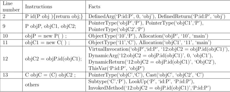
(13) • V arP ointsT o(pointer : P, heap : H) • CallGraph(invo : I, method : M ). • InterM ethAssign(to : P, f rom : P ) • Reachable(method : M ). The variable set is all the above predicate parameters. The input predicates encode analyzed program’s instructions. For example, Allocation(var, heap, inMeth) represents object allocation instructions. A new heap object, heap, is assigned to the variable, var, in the method, inM eth. Assign, Load, Store, VirtualInvocation respectively represents assigning, object-field loading, object-field storing and method invocation. Def inedArg encodes the local parameters of the method meth and DynamicArg encodes the variables passed to method meth by an invocation invo. Similarly, DefinedReturn and DynamicReturn encode the local return variable and the return object of the invocation invo. The Subtype denotes superclass relation from Definition 1.2.1. Note that our points-to analysis supports on-the-fly call graph computation so that a method invocation described by V irtualInvocation is a virtual call. The analyzed facts (instances of the analyzed predicates) are the intermediate tuples and the output of the points-to analysis. For example, V arP ointsT o tuples are the main output (the set P in the definition 1.2.2). Those analyzed facts are created by repeatedly applying analysis rules from the input facts. Consider the example 1.1.1, the input facts Table 2.1: The input facts for the example 1.1.1 Line Instructions Facts number 2 P id(P obj ){return obj;} DefinedArg(‘P:id:P’, 0, ‘obj’), DefinedReturn(‘P:id:P’, ‘obj’) PointerType(‘objP’,‘P’), PointerType(‘objC1’,‘P’), 9 P objP, objC1, objC2; PointerType(‘objC2’,‘P’) 10 objP = new P( ) ; ObjectType(‘10’,‘P’), Allocation(‘objP’, ‘10’, ‘main’) 11 objC1 = new C( ) ; ObjectType(‘11’,‘C’), Allocation(‘objC1’, ‘11’, ‘main’) VirtualInvocation(‘objP’,‘id:P’, ‘12:objC2 = objP.id(objC1)’), DynamicArg(‘12:objC2 = objP.id(objC1)’, 0, ‘objC1’), 12 objC2 = objP.id(objC1); DynamicReturn(‘12:objC2 = objP.id(objC1)’, ‘ObjC2’), ThisVar(‘P:id:P’, ‘objP’) 13 C objC = (C) objC2 ; PointerType(‘objC’,‘C’), Cast(‘objC’, ‘objC2’, ‘C’) Subtype(‘C’,‘P’), LookUp(‘P’, ‘id:P’, ‘P:id:P’), others InvokedMethod(‘12:objC2 = objP.id(objC1)’,‘P:id:P’) are shown in Table 2.1. ‘P : id : P ’ is the method signature for the function id of class P with one parameter which has type P . ‘12 : objC2 = objP.id(objC1)’ is a method invocation. An instruction can be simply represented by its line number. Hence, the heap allocations are denoted as line numbers, {‘10’, ‘11’}. After analyzing, the analyzed facts are listed below.. 7.

(14) V arP ointsT o(‘objP ’, ‘10’) V arP ointsT o(‘objC2’, ‘11’) V arP ointsT o(‘obj’, ‘11’) InterM ethAssign(‘obj’, ‘objC1’) Reachable(‘main’). V arP ointsT o(‘objC1’, ‘11’) V arP ointsT o(‘objC’, ‘11’) CallGraph(‘12:objC2 = objP.id(objC1)’, ‘P : id : P ’) InterM ethAssign(‘objC2’, obj) Reachable(‘P : id : P ’). The simple points-to analysis rules are in Example 2.2.2. I used it to demonstrate how actually the analysis runs.. Example 2.2.2 (The simple points-to analysis rules). (1) V arP ointsT o(var, heap) ← Allocation(var, heap, inM eth). (2) V arP ointsT o(to, heap) ← Assign(to, f rom), V arP ointsT o(f rom, heap). (3) V arP ointsT o(to, heap) ← InterM ethAssign(to, f rom), V arP ointsT o(f rom, heap). (4) V arP ointsT o(to, heap) ← Cast(to, f rom, type), V arP ointsT o(f rom, heap). (5) CallGraph(invo, toM eth) ← V irtualInvocation(base, sig, invo, inM eth), V arP ointsT o(base, heap), ObjectT ype(heap, heapT ), LookU p(heapT, sig, toM eth). (6) InterM ethAssign(to, f rom) ← Def inedArg(meth, n, to), DynamicArg(invo, n, f rom), CallGraph(invo, meth). (7) InterM ethAssign(to, f rom) ← Def inedReturn(meth, f rom), DynamicReturn(invo, f rom), CallGraph(invo, meth). (8) Reachable(‘main’) ← . (9) Reachable(meth) ← Reachable(inM eth), CallGraph(invo, inM eth), InvokedM ethod(inM eth, meth) Two first VarPointsTo tuples are created from the Alloc tuples. V arP ointsT o(‘objP ’, ‘10’) ← Allocation(‘objP ’, ‘10’, ‘main’). V arP ointsT o(‘objC1’, 111’) ← Allocation(‘objC1’, ‘11’, ‘main’). After applying rules (5), (6) and (7), two InterM ethAssign tuples are derived, InterM ethAssign(‘obj’, ‘objC1’) and InterM ethAssign(‘objC2’, ‘obj’). Then, rule (3) is applied twice. V arP ointsT o(‘obj’, ‘11’) ← InterM ethAssign(‘obj’, ‘objC1’), V arP ointsT o(‘objC1’, ‘11’). V arP ointsT o(‘objC2’, ‘11’) ← InterM ethAssign(‘objC2’, ‘obj’), V arP ointsT o(‘obj’, ‘11’). Finally, the last V arP ointsT o tuple comes from rule (4). V arP ointsT o(‘objC’, ‘11’) ← Cast(‘objC’, ‘objC2’, ‘C’), V arP ointsT o(‘objC2’, ‘11’). In addition, Cast(‘objC’, ‘objC2’, ‘C’) is a downcast because of P ointerT ype(‘objC2’, ‘P ’) and Subtype(‘C’, ‘P ’). Moreover, this downcast is not a fail downcast because there is only VarPointsTo(‘objC2’, ‘11’).. 8.

(15) 2.3. Context-sensitive points-to analysis. This section talks about how to deal with method call sequence, looping method call or especially recursive. Consider the simple Java program in Example 2.3.1 below. Example 2.3.1 (A simple Java program with method calls). 1 2 3 4 5 6 7 8 9 10 11 12 13 14 15 16 17. public c l a s s P{ P i d (P o b j ) { return o b j ; } } public c l a s s C extends P{ void d o n o t h i n g ( ) {} } public c l a s s M{ public s t a t i c void main ( S t r i n g [ ] a g r s ) { P objP1 , objP2 , objC1 , objC2 ; objP1 = new P ( ) ; objC1 = new C( ) ; objC2 = objP1 . i d ( objC1 ) ; objP2 = objP1 . i d ( objP1 ) ; C objC = (C) objC2 ; C objP = (C) objP2 ; } }. By applying the simple points-to analysis rules in Example 2.2.1, it is easy to compute InterM ethAssign(‘obj’, ‘objC1’), InterM ethAssign(‘objC2’, ‘obj’), InterM ethAssign(‘obj’, ‘objP 1’), and InterM ethAssign(‘objP 2’, ‘obj’). Then, V arP ointsT o(‘objC2’, ‘10’), V arP ointsT o(‘objC2’, ‘11’), V arP ointsT o(‘objP 2’, ‘10’), andV arP ointsT o(‘objP 2’, ‘11’) are derived. But, it is clearly seen that variable objC2 only points to ‘11’ and variable objP 2 only points to ‘10’. This failure is made because two method invocation at line 12 and 13 are treated under the same context. The tuples in the two pairs below (InterM ethAssign(‘obj’, ‘objC1’), InterM ethAssign(‘objP 2’, ‘obj’), ) and (InterM ethAssign(‘obj’, ‘objP 1’), InterM ethAssign(‘objC2’, ‘obj 0 ’), ) do not coexist. In order to encode this kind of information, straightforwardly a context term is added to the predicates. Basically, each method invocation must have a distinguished context. These contexts encode the scope of pointers (local variables and object fields). An instance of the pointer (variable) is cloned for each context. For example, there should be two different instances of obj for two method invocations at line 12 and 13. Additionally, there are two kinds of context, local-variable context (shortly context) and heap context. The context and heap context are respectively used for local variables and object fields. 9.

(16) Definition 2.3.1. Context and heap context (HContext) in context-sensitive analysis are defined as follows: Context = HContext = Lab∗ where Lab is the set of line numbers. Example 2.3.2 (A simple context-sensitive points-to analysis program’s components [12]). Two following constants set are added. • C is a set of (local-variable) contexts • HC is a set of heap contexts The input predicates are similar to Example 2.2.1. The analyzed predicates are: • V arP ointsT o(var : V, ctx : C, heap : H, hctx : HC) • CallGraph(invo : I, callerCtx : C, meth : M, calleeCtx : C) • InterM ethAssign(to : V, toCtx : C, f rom : V, f romCtx : C) • Reachable(meth : M, ctx : C) Additionally, there are two functions: • Record(heap : H, ctx : C) = newHCtx : HC • M erge(heap : H, hctx : HC, invo : I, ctx : C) = newCtx : C The atoms of a context-sensitive points-to analysis are shown in Example 2.3.2. In comparison to the Example 2.2.1, two context sets, C and HC, are added. The input predicates are the same, it means that we have no change in the input tuples. All analyzed predicates become context-sensitive and they are inserted by contexts. The InterM ethAssign predicate becomes InterM ethAssign(to, toContext, f rom, f romContext) where toContext and fromContext are the contexts related to variables to and f rom respectively. For the output predicates, V arP ointsT o(var, ctx, heap, hctx), the context ctx and the var identify a cloned variable for the variable var in the context ctx. Similarly, (heap, hctx) pair denotes a cloned heap of the object created at heap in the heap context hctx. Definition 2.3.2. M erge and Record functions are defined as follows: Record ∈ Record : Lab × Context → HContext M erge ∈ Merge : Lab × HContext × Lab × Context → HContext where Lab is the set of line numbers.. 10.

(17) The constants are mostly created at the parsing phase (i.e. the constants in Example 2.2.1 are produced in the parsing phase), but contexts instances are generated while the analysis rules are applied (inference). The Merge function constructs contexts and the Record function constructs heap contexts (the basic Datalog language does not have the function but some variant have). They are in Definition 2.3.2. Note that heap and invo in Example 2.3.2 are the line numbers. A heap context is created when a new object is allocated with a heap allocation. A method invocation requires a scope identifier for the local variables, then a context is constructed by the Merge function. See Example 2.3.3. Example 2.3.3 ( The simple context-sensitive points-to analysis rules). (1) Record(heap, ctx) = hctx, V arP ointsT o(var, ctx, heap, hctx) ← Allocation(var, heap, inM eth). (2) V arP ointsT o(to, ctx, heap, hctx) ← Assign(to, f rom), V arP ointsT o(f rom, ctx, heap, ctx). (3) V arP ointsT o(to, toCtx, heap, hctx) ← InterM ethAssign(to, toCtx, f rom, f romCtx), V arP ointsT o(f rom, f romCtx, heap, hctx). (4) V arP ointsT o(to, ctx, heap, hctx) ← Cast(to, f rom, type), V arP ointsT o(f rom, ctx, heap, hctx). (5) M erge(heap, hctx, invo, callerCtx) = calleeCtx, CallGraph(invo, callerCtx, toM eth, calleeCtx) ← V irtualInvocation(base, sig, invo, inM eth), V arP ointsT o(base, callerCtx, heap, hctx), ObjectT ype(heap, heapT ), LookU p(heapT, sig, toM eth). (6) InterM ethAssign(to, calleeCtx, f rom, callerCtx) ← Def inedArg(meth, n, to), DynamicArg(invo, n, f rom), CallGraph(invo, callerCtx, meth, calleeCtx). (7) InterM ethAssign(to, callerCtx, f rom, calleeCtx) ← Def inedReturn(meth, f rom), DynamicReturn(invo, f rom), CallGraph(invo, callerCtx, meth, calleeCtx). Finally, I give an example of the Merge and Record functions as below. record(heap, ctx) = ctx merge(heap, hctx, invo, ctx) = ctx ⊕ invo where ⊕ is the concatenating operator. Now, we run the context-sensitive analysis program above on the simple Java program in Example 2.3.1. The contexts are three callgraph paths ‘0’ (for the main method execution), ‘0, 12’ (for the first id function invocation at line 12) and ‘0, 13’ (for the second one). I use line number 0 to demonstrate the main function call. Then, there are (InterM ethAssign(‘obj’, ‘0, 13’, ‘objP 1’, ‘0’), InterM ethAssign(‘objP 2’, ‘0’, ‘obj’, ‘0, 13’), ) and (InterM ethAssign(‘obj’, ‘0, 12’, ‘objC1’, ‘0’), InterM ethAssign(‘objC2’, ‘0’, ‘obj’, ‘0, 12’), ). 11.

(18) So that, two data flows, objP 1 → obj → objP 2 and objC1 → obj → objC2, have been separated. Additionally, the simple points-to analysis in Example 2.2.2 is a contextinsensitive analysis.. 2.4. Call-site sensitivity, object sensitivity and type sensitivity. Our context-sensitive analysis is cloning approach in which the analyzed program’s components (variable, objects) are cloned for each context. Many kinds of context are defined, such as call-site, object, type [1]. Besides the methods that use a single kind of context, a hyper approach have been proposed [10] by a combination.. 2.4.1. Call-site sensitivity. By changing the definition of Context, HContext and two manipulating functions (Record and Merge), a type of context-sensitive analysis is established. In Section 2.3, I defined a call-site-sensitive analysis. Context and HContext are sequences of labels, label ∈ Lab, where the labels are line numbers of method call instructions (12 and 13 in Example 2.3.1). Record(heap, ctx) = ctx. A heap context of an allocated object is the call-site (context) of the caller. The Merge function concatenates the caller’s call site with the current callsite (for example, M erge(‘10’, ‘0’, ‘12’, ‘0’) = ‘0, 12’). I remark that the contexts in the call-site sensitive analysis are sequences of call-sites and they also are the call paths in call-graph. Also, hcontexts are sequences of call-site line numbers.. 2.4.2. Object sensitivity and type sensitivity. The call-site-sensitive points-to analysis divides contexts by calling chains. Besides, the object sensitivity has been proposed [1] as an another way to divide contexts. The objectsensitive analysis is suggested to work well for object-oriented programs. Definition 2.4.1. Context and heap context (HContext) in object-sensitive analysis are as follows: Context = HContext = Lab∗ where Lab is the set of line numbers of heap allocation instructions. Example 2.4.1. Record and Merge in object-sensitive analysis are defined as follows: Record(heap, ctx) = ctx M erge(heap, hctx, invo, ctx) = hctx ⊕ heap A context now is a sequence of heap allocation line numbers. It starts from ‘0’, which denotes the heap allocation of the object of M ain class. On the other way, variables are cloned based on base object’s creation. For example, in this instruction base.meth(args), 12.

(19) the context inside meth method invocation is identified by the allocation of the base object. For understanding, see the following example. Example 2.4.2 (A simple Java program with method calls). 1 2 3 4 5 6 7 8 9 10 11 12 13 14 15 16 17 18. public c l a s s P{ P i d (P o b j ) { return o b j ; } } public c l a s s C extends P{ void d o n o t h i n g ( ) {} } public c l a s s M{ public s t a t i c void main ( S t r i n g [ ] a g r s ) { P objP1 , objP2 , objC1 , objC2 , objC3 ; objP1 = new P ( ) ; objC1 = new C( ) ; objC2 = objC1 . i d ( objC1 ) ; objP2 = objP1 . i d ( objP1 ) ; objC3 = objC1 . i d ( objC1 ) ; C objC = (C) objC2 ; objC = (C) objC3 ; } }. Three method invocations at lines 12, 13 and 14 are only considered under two different contexts. 12 and 13 will have the same context; because line 12 and line 14 have the same base object created at line 11 (objC1 = newC();). In this case, the object-sensitive analysis is still precise enough to conclude that two downcasts at line 15 and 16 are safe. However, if line 14 is modified to become objC3 = objP 1.id(objC1);, the analysis will fail to prove the safety of the second downcast. At this point, it seems that object sensitivity is always worse than call-site sensitivity. But it not true. The next section shows that there are cases where an object-sensitive points-to analysis works better than a call-sensitive one. In general, the object-sensitive points-to analysis is more scalable than the call-sensitive analysis. In 2011, a type-sensitive analysis was proposed by Yannis et. al. [1]. It also takes the object-oriented concept, likes object-sensitive analysis. Type-sensitive analysis has higher scalability than object-sensitive analysis but is less precise. Definition 2.4.2. Context and heap context (HContext) in type-sensitive analysis are as follows: Context = HContext = T ype∗ where T ype is the set of class types. The type-sensitive contexts are defined above. The manipulating functions only keep the type information instead of heap allocation. Example 2.4.3. Record(heap, ctx) = ctx M erge(heap, hctx, invo, ctx) = hctx ⊕ T ypeOf (heap) where T ypeOf (·) returns type of the created object. 13.

(20) 2.5. Abstraction. In order to precisely handle (recursive) call sequence, the context should simply be full call path. Hence, the context is defined as the sequence of line number in Definition 2.3.1. However, the contexts will become infinite and our analysis will be undecidable. To this end, k-context-sensitive analysis [2] abstracts contexts to be finite as follows. Definition 2.5.1. Context and HContext in k-context- h-heap context- sensitive analysis are as follows: Context = Labk , HContext = Labh . A bounded version of contexts is described in Definition 2.5.1. Often, only (small) bounded length contexts are sufficient. Two manipulating functions, Record and Merge are also changed. Example 2.5.1. Two manipulating functions of a k-context- h-heap context- sensitive analysis are as follows: Record(heap, ctx) = lasth (ctx) M erge(heap, hctx, invo, ctx) = lastk (ctx ⊕ invo) where the lastn (s) function returns the n last elements of the sequence s. Consider Example 2.3.1, a 1-context-sensitive points-to analysis is precise enough to distinguish two invocations of the id method. First, there are Record(‘10’, ‘0’) = ‘0’, V arP ointsT o(‘objP 1’, ‘0’, ‘10’, ‘0’) ← Allocation(‘objP 1’, ‘10’, ‘main’)., Record(‘11’, ‘0’) = ‘0’, V arP ointsT o(‘objC1’, ‘0’, ‘11’, ‘0’) ← Allocation(‘objC1’, ‘11’, ‘main’)., M erge(‘10’, ‘0’, ‘12’, ‘0’) = ‘12’, CallGraph(‘12’, ‘0’, ‘P : id : P ’, ‘12’) ← V irtualInvocation(‘objP 1’, ‘0’, ‘12’, ‘main’), V arP ointsT o(‘objP 1’, ‘0’, ‘10’, ‘0’), ObjectT ype(‘10’, ‘P ’), LookU p(‘P ’, ‘id : P ’, ‘P : id : P ’). and M erge(‘11’, ‘0’, ‘13’, ‘0’) = ‘13’, CallGraph(‘13’, ‘0’, ‘P : id : P ’, ‘13’) ← V irtualInvocation(‘objP 1’, ‘0’, ‘13’, ‘main’), V arP ointsT o(‘objP 1’, ‘0’, ‘10’, ‘0’), ObjectT ype(‘10’, ‘P ’), LookU p(‘P ’, ‘id : P ’, ‘P : id : P ’). Then, there are (InterM ethAssign(‘obj’, ‘13’, ‘objP 1’, ‘0’), InterM ethAssign(‘objP 2’, ‘0’, ‘obj’, ‘13’), ) and (InterM ethAssign(‘obj’, ‘12’, ‘objC1’, ‘0’), InterM ethAssign(‘objC2’, ‘0’, ‘obj’, ‘12’), ).. 14.

(21) Chapter 3 Proposed method 3.1. Adaptive points-to analysis. Consider the following Java program. Example 3.1.1 (A simple Java program for selective points-to analysis). 1 2 3 4 5 6 7 8 9 10 11 12 13 14 15 16 17 18 19 20 21. public c l a s s P{} public c l a s s C extends P{} public c l a s s M{ public s t a t i c void main ( S t r i n g [ ] a g r s ) { P objP , objC , objP1 , objP2 , objP3 ; objP = new P ( ) ; objC = new C( ) ; objP1 = fun1 ( objP ) ; objP2 = fun1 ( objC ) ; objP3 = fun2 ( objP ) ; objP3 = fun2 ( objC ) ; (C) objP1 ; // downcast ‘ d1 ’ (C) objP2 ; // downcast ‘ d2 ’ (C) objP3 ; // downcast ‘ d3 ’ } public s t a t i c P fun1 (P o b j 1 ) { return i d ( o b j 1 ) ; } public s t a t i c P fun2 (P o b j 2 ) { C temp = new C( ) ; return i d ( temp ) ; } public s t a t i c P i d (P o b j ) { return o b j ; } }. Let us analyze it with the 2-call-site sensitive points-to analysis mentioned in Chapter 2. The result contains V arP ointsT o(‘objP ’, ‘0’, ‘6’, ‘0’), V arP ointsT o(‘objC’, ‘0’, ‘7’, ‘0’), V arP ointsT o(‘objP 1’, ‘0’, ‘6’, ‘0’),. V arP ointsT o(‘objP 2’, ‘0’, ‘7’, ‘0’), V arP ointsT o(‘objP 3’, ‘0’, ‘18’, ‘0, 10’), V arP ointsT o(‘objP 3’, ‘0’, ‘18’, ‘0, 11’).. Therefore, the first downcast at line 12 fails and two remaining are safe. These are the precise result. On the other hand, if we analyze the above Java program with a 1-call-site 15.

(22) sensitive points-to analysis, the analyzed tuples are quite different. V arP ointsT o(‘objP ’, ‘0’, ‘6’, ‘0’), V arP ointsT o(‘objC’, ‘0’, ‘7’, ‘0’), V arP ointsT o(‘objP 1’, ‘0’, ‘6’, ‘0’), VarPointsTo(‘objP1’, ‘0’, ‘7’, ‘0’),. VarPointsTo(‘objP2’, ‘0’, ‘6’, ‘0’), V arP ointsT o(‘objP 2’, ‘0’, ‘7’, ‘0’), V arP ointsT o(‘objP 3’, ‘0’, ‘18’, ‘10’), V arP ointsT o(‘objP 3’, ‘0’, ‘18’, ‘11’).. The differences make a failure when proving the safety of the second downcast. For this Java program, a level 1 abstraction is precise enough to analyze the behavior of f un2, but the method invocations of the f un1 need level 2. This leads to the idea that we should handle different parts of the program with different abstraction levels. This section introduces an adaptive context-sensitive points-to analysis, which is able to handle the parts of the program selectively. Firstly, I define the contexts in Definition 3.1.1. Context and HContext are sets of the following context and hcontext respectively. Definition 3.1.1 (context and heap context in adaptive k-context- h-heap context- sensitive analysis). context = lab1 , ..., labα. hcontext = lab1 , ..., labβ. where 0 ≤ α ≤ k, 0 ≤ β ≤ h and lab ∈ Lab (set of line numbers). Definition 3.1.2. M erge and Record functions in adaptive k-context- h-heap contextsensitive analysis are as follows: Record ∈ Record : Lab × Context × HAbs → HContext M erge ∈ Merge : Lab × HContext × Lab × Context × Abs → HContext where Abs = [z...k], HAbs = [z...h], and z is the smallest abstraction level, e.g. z = 1. The abstraction levels are added into two manipulating functions. Then the abstraction levels no longer are two numbers, k and h. From now, abstraction describes the abstraction levels for parts of the analyzed program. Definition 3.1.3. abstraction and heap abstraction in adaptive k-context- h-heap contextsensitive analysis are as follows: abstraction = abs1 , ..., absn heapAbstraction = habs1 , ..., habsm where abs ∈ Abs, habs ∈ HAbs, and n and m are numbers of the analyzed program’s parts. In detail, our method divides the program by instruction. Hence, n and m are the numbers of method invocations and heap allocations respectively. An abstraction for the program in Example 3.1.1 is ‘1,1,1,1,2,1’ (corresponding with the method invocations 16.

(23) at lines 8, 9, 10, 11, 16, 18). With it, the program is analyzed precisely. In addition, ‘1,1,1,1,2,1’ is also the least precise abstraction that can prove all downcasts in the above program. In the rest of this document, only context and abstraction is mentioned in the examples. The hcontext and heapAbstraction are hidden for simplifying the examples. Definition 3.1.4 (Abstraction comparison). An abstraction A is more precise than an abstraction B, if and only if Ai < Bi for any pair (Ai ∈ A, Bi ∈ B). 3.2. Problem restatement. In fact, an adaptive k-context- h-heap context- sensitive analysis is not more precise than a k-context- h-heap context- sensitive analysis. The equality happens with highest abstractions (‘k, k, .., k’ and ‘h, h, ..., h’). In my experiment, 3-context- 3-heap contextsensitive analysis is not achievable because of state explosion. Therefore, I propose obtaining the precision of a high-abstracted analysis by running the adaptive analysis with lower abstractions. The downcast problem is simply restated as below. Definition 3.2.1 (The downcast problem). Given a Java program P , a set D of downcasts and a valid abstraction set A. Compute a partition (T , F ) of D, where T contains down casts that can be proved by some valid abstraction A ∈ A and F is a set of down casts that may fail.. 3.3. CEGAR-based algorithm. In order to solve the downcast problem, a CEGAR-based algorithm has been proposed by Zhang et. al [2]. The CEGAR-based algorithm is shown in Algorithm 1. CEGAR iteration starts by running the adaptive analysis with the lowest abstraction. After every analyzing step, the counterexample knowledge is accumulated. It is used to choose an abstraction for the next iteration. The key points are the way to represent the counterexample knowledge φ and how it can guide the abstraction refinement (the choose function). I define φ and choose later. To give an early taste, I describe how the CEGAR-based algorithm works on Example 3.1.1 with an adaptive 2-call-site sensitive points-to analysis (h = k = 2). First, The analysis starts with the lowest abstraction, a1 = ‘1, 1, 1, 1, 1, 1’. There are V arP ointsT o(‘objP ’, ‘0’, ‘6’, ‘0’), V arP ointsT o(‘objC’, ‘0’, ‘7’, ‘0’), V arP ointsT o(‘objP 1’, ‘0’, ‘6’, ‘0’), V arP ointsT o(‘objP 1’, ‘0’, ‘7’, ‘0’),. V arP ointsT o(‘objP 2’, ‘0’, ‘6’, ‘0’), V arP ointsT o(‘objP 2’, ‘0’, ‘7’, ‘0’), V arP ointsT o(‘objP 3’, ‘0’, ‘18’, ‘10’), V arP ointsT o(‘objP 3’, ‘0’, ‘18’, ‘11’);. and fail downcasts: F ailDownCast(‘objP 1’, ‘’, ‘C’),. F ailDownCast(‘objP 2’, ‘’, ‘C’).. The lowest abstraction means that there is a single context,‘0’, for everywhere. The counterexample knowledge is a chain of inferences. For the first downcast, 17.

(24) Algorithm 1 CEGAR-based algorithm Input: Program P and downcasts D Output: A partition (T, F ) of D, where T contains the downcastings that will not fail and F is set of the down-casting that may fail. a := ⊥ // as initial abstraction (lowest-precision) φ := {} // φ is accumulated counter-example and initiated as empty set T := {} and F := D loop φ, (T 0 , F 0 ) = Analyze(F, a) // invoke the analysis T := T ∪ T 0 F := F 0 a := choose(φ, F ) end loop F ailDownCast(‘objP 1’, ‘’, ‘C’) ← V arP ointsT o(‘objP 1’, ‘0’, ‘6’, ‘0’), Cast(‘objP 1’, ‘’, ‘C’). V arP ointsT o(‘objP 1’, ‘0’, ‘6’, ‘0’) ← InterM ethAssign(‘objP 1’, ‘0’, ‘id(obj1)’, ‘8’), V arP ointsT o(‘id(obj1)’, ‘8’, ‘6’, ‘0’). V arP ointsT o(‘id(obj1)’, ‘8’, ‘6’, ‘0’) ← InterM ethAssign(‘id(obj1)’, ‘8’, ‘obj’, ‘16’), V arP ointsT o(‘obj’, ‘16’, ‘6’, ‘0’). V arP ointsT o(‘obj’, ‘16’, ‘6’, ‘0’) ← InterM ethAssign(‘obj’, ‘16’, ‘obj1’, ‘8’), V arP ointsT o(‘obj1’, ‘8’, ‘6’, ‘0’). V arP ointsT o(‘obj1’, ‘8’, ‘6’, ‘0’) ← InterM ethAssign(‘obj1’, ‘8’, ‘objP ’, ‘0’), V arP ointsT o(‘objP ’, ‘0’, ‘6’, ‘0’). and InterM ethAssign(‘objP 1’, ‘0’, ‘id(obj1)’, ‘8’) and InterM ethAssign(‘obj1’, ‘8’, ‘objP ’, ‘0’) are consequences of Abs(‘8’, 1). Abs(‘n’, abs) means that the method invocation at line n is abstracted with level abs. InterMethAssign( ‘id(obj1)’, ‘8’, ‘obj’, ‘16’) and InterMethAssign(‘obj’,‘16’, ‘obj1’, ‘8’) are consequences of Abs(‘16’, 1). The similar thing happens with the second downcast. Finally, there are two rules below. F ailDownCast(‘objP 1’, ‘’, ‘C’) ← ..., Abs(‘8’, 1), Abs(‘16’, 1). F ailDownCast(‘objP 2’, ‘’, ‘C’) ← ..., Abs(‘9’, 1), Abs(‘16’, 1). The choose function takes φ and F as the inputs. At this point, F includes two first downcasts. The above inference chains say that • F ailDownCast(‘objP 1’, ‘’, ‘C’) may not exist if Abs(‘8’, 1) or Abs(‘16’, 1) dose not exist. • F ailDownCast(‘objP 2’, ‘’, ‘C’) may not exist if Abs(‘9’, 1) or Abs(‘16’, 1) dose not exist. 18.

(25) For example, the choose function returns a2 = ‘1, 1, 1, 1, 2, 1’ as the abstraction for the second iteration. Then, only F ailDownCast(‘objP 1’, ‘’, ‘C’) remains. The counterexample knowledge now says • F ailDownCast(‘objP 1’, ‘’, ‘C’) is produced for any abstraction b = ‘b1 , b2 = 1, b3 , b4 , b5 , b6 ’. • F ailDownCast(‘objP 1’, ‘’, ‘C’) is also produced by any abstraction b = ‘b1 , b2 = 1, b3 , b4 , b5 = 1, b6 ’. The second iteration returns abstraction a3 = ‘1, 2, 1, 1, 1, 1’ and the third returns a4 = ‘1, 2, 1, 1, 2, 1’. However, F ailDownCast(‘objP 1’, ‘’, ‘C’) still exists. Recall that the maximum abstraction level is 2. Hence the CEGAR-based algorithms stops after the fourth iteration. The final result is (T = {‘d2’, ‘d3’}, F = {‘d1’}).. 3.3.1. Choosing abstraction with by maximum satisfiability (MaxSAT). In this subsection, the choose function is defined as a partial weighted MaxSAT problem. Definition 3.3.1 (MaxSAT). MaxSAT is SAT with soft constraints (pairs of clause and weight). Its goal is to find a model that maximizes the sum of satisfied soft constraints’ weight. Note that, our points-to analysis is implemented in Datalog language, and it is in predicate logic. However, MaxSAT is a binary (propositional) logic problem. Therefore, any tuple needs to be converted to a variable. For example, the abstraction a = ‘1, 1, 1, 1, 1, 10 is encoded as [a1 = 1] ∧ [a2 = 1] ∧ [a3 = 1] ∧ [a4 = 1] ∧ [a5 = 1] ∧ [a6 = 1] where [ai = 1] is a boolean variable. In the previous CEGAR-based algorithm explanation, the counterexample knowledge φ after the second iteration is ([a2 = 1] → [F ailDownCast(‘objP 1’, ‘’, ‘C’)]) or (¬[a2 = 1] ∨ [F ailDownCast(‘objP 1’, ‘’, ‘C’)]). The choose function is formulated as below. Definition 3.3.2 (The choose(φ, F ) function). choose(φ, F ) = M axSAT (A ∧ α(F ) ∧ φ, γa ∧ WF ) where A ∧ α(F ) ∧ φ is the hard constraint and γa ∧ WF is the soft constraint. In details, • A represents the valid abstraction. A = {[ai = z] ∨ [ai = z + 1]) ∨ ... ∨ [ai = k]| 1 ≤ i ≤ n}; where z is the minimum abstraction level, k is the maximum abstraction level and n is the number of parts of the analyzed program. V. • φ encodes the accumulated counter-example knowledge. See Section 3.4. 19.

(26) • The α(F ) = {¬[d]| d ∈ F } constraint says that there has to be at least one downcast to be proved by the chosen abstraction. V. • γa denotes the complexity order of the abstraction levels. γa is a set of ([ai = level], w) tuples. The higher abstraction level has the lower weight. • WF = {([d], maxw)| d ∈ F } where maxw > sum({w| ([ai = k], w) ∈ γa }) and k is the maximum abstraction level. The WF constraint enforces that the solution actually proves at least one downcast in F . Definition 3.3.3 (Valid abstraction). A = ‘a0 , a1 , ..., an ’ is a valid abstraction of a program P with an adaptive k-context-sensitive points-to analysis, iff z < ai < k for 0 < i < n. Theorem 3.3.1. If M axSAT (A ∧ α(F ) ∧ φ, γa ∧ WF ) returns no solution; then there is no valid abstraction which can prove a downcast in F . Consider Theorem 3.3.1, if a MaxSAT solver gives no solution, it means that there is no model which can satisfy A ∧ α(F ) ∧ φ. Hence, no downcast in F can be proved by a valid abstraction. However, some downcasts in F might be still safe, and it can be proved by some abstractions that are more precise than the highest abstraction (‘k, k, ..., k’). The CEGAR-based algorithm will terminate if the choose function returns no valid abstraction. Theorem 3.3.2. The CEGAR-based algorithm with an adaptive k-context-sensitive points-to analysis solves the downcast problem and gives the same precise results as a k-context-sensitive points-to analysis does.. 3.4. Provenances vs Datalog runs. In the previous section, the counterexample knowledge φ is mentioned as inference chains. More precisely, φ is a set of analysis rule applications. According to the notations in the definitions in Section 2.1, a rule is l0 ← l1 , .., ln ; then a rule application is σ(l0 ) ← σ(l1 ), .., σ(ln ) where σ(l0 ), σ(l0 ), ..., σ(ln ) ∈ T and T is the produced tuples set. The counterexample knowledge was defined as a set of provenances in [2]; but in our method, I propose to use the set of Datalog runs as the counterexample knowledge. Definition 3.4.1 (Datalog runs). The set of Datalog runs produced by a Datalog program C is [C]T =. ^. {σ(l0 ) ← σ(l1 ), .., σ(ln )| (l0 ← l1 , .., ln ) ∈ C and σ(l0 ), ..., σ(ln ) ∈ T }. Definition 3.4.2 (Provenance). The set of provenances |C|T is the biggest subset of [C]T that satisfies ∀σ(r) ∈ |C|T 6 ∃σ 0 (r0 ) ∈ |C|T σ(l0 ) = σ 0 (l00 ) 0 where r, r0 ∈ C, σ(r) = σ(l0 ) ← σ(l1 ), .., σ(ln ) and σ 0 (r0 ) = σ 0 (l00 ) ← σ 0 (l10 ), .., σ 0 (lm ).. 20.

(27) The same tuple can be produced by applying two or more rules. Provenances only keep the information of the first-producing rule application, while it skips the applications that create any existing tuple. Differently, Datalog runs save all the producing relations. Therefore, the Datalog-run counterexample has a higher precision than the provenance counterexample, and obviously, pays a higher cost.. 3.5. Cheap abstraction for refinement. It is not necessary to run the refinement step on the same abstraction with the analysis step. It is mostly because of the computation cost. The counterexample knowledge can be modeled with a lower abstraction. Definition 3.5.1. Datalog runs with lower level abstraction is defined as follows: [C]0T =. ^. {f (σ(l0 )) ← f (σ(l1 )), .., f (σ(ln )).| (l0 ← l1 , .., ln .) ∈ C and σ(l0 ), ..., σ(ln ) ∈ T }. where f is a context lowering mapping function. For example, the Datalog run below is produced by 2-call-site-sensitive analysis. V arP ointsT o(‘objP 1’, ‘0’, ‘6’, ‘0’) ← InterM ethAssign(‘objP 1’, ‘0’, ‘id(obj1)’, ‘0,8’), V arP ointsT o(‘id(obj1)’, ‘0,8’, ‘6’, ‘0’). Then context constants are mapped to 1-length context. V arP ointsT o(‘objP 1’, ‘0’, ‘6’, ‘0’) ← InterM ethAssign(‘objP 1’, ‘0’, ‘id(obj1)’, ‘8’), V arP ointsT o(‘id(obj1)’, ‘8’, ‘6’, ‘0’). Lower context-level counterexample knowledge means that the refinement step is processed with a lower abstraction. It may lead to the false positive results, but at least it still remains sound. As with the abstract semantic, there is a trade-off between precision and analysis cost. Note that a higher level abstraction for refinement makes no sense.. 3.6. Partitioned abstraction search. In my experiment, it is too costly to use the MaxSAT solver directly for choosing the abstraction. Hence, I propose a partitioned abstraction search method with a new choose0 function below. Definition 3.6.1. With a partition (D0 , ..., Dn ) of F , choose0 (φ, F ) =. G. {choose(φ, Di )|i = 1, ..., n}. where Di is a set of downcasts and ∪ is abstraction joining operator. Definition 3.6.2 (The abstraction joining operator). With two abstractions, A = A1 , A2 , ..., An and B = B1 , B2 , ..., Bn , A t B = C = C1 , C2 , ..., Cn where Ci = max(Ai , Bi ). 21.

(28) The operation, A t B, returns the least abstraction C that is more precise than A and B. Our method applies the MaxSAT solver on smaller sub-problems. The original MaxSAT problem is solved approximately. Theorem 3.6.1. If choose0 (φ, F ) = A then A is a model of A ∧ α(F ) ∧ φ where choose(φ, F ) = M axSAT (A ∧ α(F ) ∧ φ, γa ∧ WF ).. 3.7. Repeated abstraction search. Consider the example in Section 3.3, after two iterations, the counterexample knowledge contains this information, φ = ([a2 = 1] → [F ailDownCast(‘objP 1’, ‘’, ‘C’)])∧ ([a2 = 1] ∧ [a5 = 1] → [F ailDownCast(‘objP 1’, ‘’, ‘C’)]). Then it requires two more iterations to know that [F ailDownCast(‘objP 1’, ‘’, ‘C’)] can not be disproved (run the analysis with two abstractions ‘1, 2, 1, 1, 1, 1’ and ‘1, 2, 1, 1, 2, 1’ respectively). At the end of the second iteration, the hard constraint is A ∧ α(F ) ∧ φ, A = ([a2 = 1] ∨ [a2 = 2]) ∧ ([a5 = 1] ∨ [a5 = 2]) ∧ ... α(F ) = ¬[F ailDownCast(‘objP 1’, ‘’, ‘C’)] and the soft constraint is γa ∧ WF , γa = ([a2 = 1], 1) ∧ ([a2 = 2], 0) ∧ ([a5 = 1], 1) ∧ ([a5 = 2], 0) ∧ ..., WF = (¬[F ailDownCast(‘objP 1’, ‘’, ‘C’)], 7). Then M axSAT (A ∧ α(F ) ∧ φ, γa ∧ WF ) returns [a1 = 1] ∧ [a2 = 2] ∧ [a3 = 1] ∧ [a4 = 1]∧[a5 = 1]∧[a6 = 1] (the abstraction ‘1, 2, 1, 1, 1, 1’). However, if it returns ‘1, 2, 1, 1, 2, 1’ instead, the CEGAR-based algorithm could end faster. To overcome the above scenario, we propose a repeated abstraction search; a choose function is defined below. Definition 3.7.1 (choose in repeated abstraction search). choose(φ, Di ) = choosej (φ, Di ) where Aj+1 = choosej+1 (φ, Di ) = Aj t choosej (φ ∧ β(Aj ), Di ) for β(Aj ) =. ^ p. aj 6= Aj (p) and β0 = true. p. and apj is a element of abstraction Aj. 22.

(29) Our repeated abstraction choosing method goes forward abstractions. At first, choose0 (φ, Di ) is the original MaxSAT problem. Then it assumes that the A0 does not prove any downcast by adding β(Aj−1 , A) into the hard constraint. A new alternative abstraction is F found. Finally, the chosen abstraction is i=1,...,j Ai . In the above example, at the end of the second iteration with j = 1, ‘1, 2, 1, 1, 2, 1’ is returned instead of ‘1, 2, 1, 1, 1, 1’. Thus, the CEGAR-base algorithm runs faster. Now the choosing abstraction statement in the Algorithm 1 becomes a := choose0 (φ, F ) =. G. {choosej (φ, Di )|i = 1, ..., n}. Theorem 3.7.1. For 0 ≤ j, if choosej (φ, Di ) = Aj and choosej+1 (φ, Di ) = Aj+1 then Aj+1 is not less precise than Aj (better or equal),. 23.

(30) Chapter 4 Related works 4.1. Pushdown system. Our points-to analysis is an instance of the reachability problem. In which input tuples encode initial states, analyzing rules are transition and output tuples at the end of inference describe reachable states. In addition, our transition system becomes finite-state by an abstraction in Section 2.5. Also, recursive method invocations are handled by approximating the infinite set of unbounded-length contexts using the finite set of bounded contexts. Another approach for handling recursive functions is the pushdown approach [8]. A pushdown system is a state transition system with an unbound stack and the pushdown static analysis can precisely handle recursive calls. The pushdown static analysis is also called context-free language (CFL) reachability [8]. It starts with initial states and then the reachable states are gradually reached. In 2001, the pushdown points-to analysis was introduced by Rehof and Fahndrich [9]. During the analyzing time, the proposed system obtains and accumulates every function behaviors. These behaviors are then encoded as mapping relations between sets of input states and sets of possible output states. In the pushdown approach, the infinite states are abstracted to a finite number of state subsets. In the points-to analysis, the maximum number of state subsets is s = p×n where p is the number of pointers and n is the number of objects. Furthermore, the mapping function is M = S × S where S is a set of state subsets. We also have that the number of functions is finite. Therefore, the pushdown static analysis is decidable. All in all, the points-to analysis with the pushdown approach is decidable. It is hard to compare the precision of this approach and our approach. However, from the performance perspective, our approach has an advantage as being more scalable [13]. In addition, our method works with antlr and chart while [13] dose not. Besides these advantages, our approach has a key drawback that is how to pick a good abstraction. The program should be analyzed with small enough number of states but still sufficient to prove the goals (downcasts). This thesis focuses on solving these problems.. 24.

(31) 4.2. Abstraction Refinement. In the previous section, we stated that the points-to analysis can be considered as a reachability problem which is decidable if the states are finite. Beside the pushdown system, there is another method that map the infinite states of the program semantic to a set of finite abstracted states by defining an abstract semantic. Our points-to analysis is influenced by this approach. Recall that the key problem with this approach is how to pick a good abstraction. There is one prominent work by Zhang et. al. [2]. They try to address this issue. In 2014, they proposed the CEGAR-based abstraction refinement [2] which models the “picking good abstraction” as a MaxSAT problem, see Subsection 3.3.1. They also proposed the usage of provenances as counter example knowledge to generalize the failure of abstractions. The cheapest refined abstraction is chosen based on these provenances. In this work, we extend [2]’s work by using a more fine-grained granularity of program parts. Namely, our approach uses different precision levels for different method call sites, whereas [2] does not. We also describes some problems we found while extending [2] in Chapter 3. Therefore, we propose the use of Datalog runs instead of provenances to gain higher precision. Finally, we suggest partition abstraction search for feasibility and repeated search for abstraction forwarding.. 25.

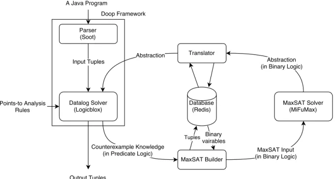
(32) Chapter 5 Implementation Our analysis system is described in Figure 5.1. Doop is a points-to analysis framework for Java programs. The Doop framework precisely handles many Java features (such as inheritance, reflection, exception). Doop includes many context-sensitive analyses (callsite-sensitive, object-sensitive and type-sensitive analyses) and it is easy to define a new analysis. Doop uses the Datalog language and Logicblox (a Datalog solver). In Doop, an input Java program is parsed into input tuples that can be used as data in a Java program by using the Soot library [4]. Logicblox, a Datalog solver, starts the analysis with those input tuples, abstraction tuples and points-to analysis rules. After the analysis, counterexample knowledge is extracted in the form of predicate tuples. There is a gap between the predicate logic (our points-to analysis) and the binary logic (MaxSAT). I use the Redis database [14] to bind them. The MaxSAT problem in Chapter 3 is solved by MiFuMax [5]. If the MaxSAT solver returns no solution (abstraction) then the CEGAR-based algorithm ends. In the following, I discuss the some relevant details of the implementation, such as optimizations that were not described in the earlier part of the thesis.. 5.1. Eliminate non-context predicates from counterexample knowledge. In order to decrease the cost of the MaxSAT problem, some redundant tuples should be removed from the counterexample knowledge. Hence, the non-context predicates are considered. Definition 5.1.1 (Non-context predicate). Non-context predicate is the predicate that does not include any context variable (Context or HContext). The analysis inference produces analyzed tuples from input tuples. There are rules that create non-context analyzed tuples. For example, SupertypeOf (?t, ?s) ← ComponentT ype[?s] =?sc, ComponentT ype[?t] =?tc, Ref erenceT ype(?sc), Ref erenceT ype(?tc), SubtypeOf (?sc, ?tc). 26.

(33) Figure 5.1: System architecture In fact, all input tuples are non-context predicates. Moreover, there is no rule such that a non-context tuple is created from context tuples. Therefore, it is simple to get the following theorem. Theorem 5.1.1. Let FC1 and FC2 be the points-to analysis rules with different abstractions for a same program. Let Ti = lf p(FCi , T0 ) for each i ∈ 1, 2 where T0 is the starting facts for the program. Let Ti0 ⊆ Ti be the set of non-context tuples of Ti (for each i ∈ 1, 2). Then, T10 = T20 . As Theorem 5.1.1, the non-context predicates are always the same, regardless of what the abstraction is. Therefore, the non-context predicates do not help to pick a good abstraction. Hence, in our implementation, the counterexample knowledge dose not include any non-context predicates, except for the abstraction predicates.. 5.2. Trace tuples from may fail downcasts. Consider the CERGAR-based algorithm in Algorithm 1, F is the remaining may-fail downcast. This set is deceasing over time. Because of computation cost, the counterexample knowledge φ ignores any downcast which does not belong to F . I manually wrote the tracing rules to extract all inferences which lead to a F ailDownCast tuple creation. The following is an example. F V arP ointsT o(?heap, ?f rom) ← ApplicationClass(?class), M ethodSignature : DeclaringT ype[?inmethod] =?class, 27.

(34) Reachable(?inmethod), Cast(?type, ?f rom, ?to, ?inmethod), V arP ointsT o( , ?heap, , ?f rom), HeapAllocation : T ype[?heap] =?heaptype, !SupertypeOf (?type, ?heaptype). The above is the tracing rule of the rule below. F ailDownCast(?f rom, ?to, ?type) ← ApplicationClass(?class), M ethodSignature : DeclaringT ype[?inmethod] =?class, Reachable(?inmethod), Cast(?type, ?f rom, ?to, ?inmethod), V arP ointsT o( , ?heap, , ?f rom), HeapAllocation : T ype[?heap] =?heaptype, !SupertypeOf (?type, ?heaptype). We use the tracing rules instead of recording because Logicblox does not support recording.. 5.3. Rewrite points-to analysis rules. In the Doop framework, there are some intermediate rules. They makes the analysis rules easy to read and understand. For example, there are: V arP ointsT o(?hctx, ?heap, ?toCtx, ?to) ← V arP ointsT o(?hctx, ?heap, ?f romCtx, ?f rom), Assign(?type, ?toCtx, ?to, ?f romCtx, ?f rom), HeapAllocation : T ype[?heap] =?heaptype, SupertypeOf (?type, ?heaptype). and Assign(?type, ?ctx, ?to, ?ctx, ?f rom) ← AssignCast(?type, ?f rom, ?to, ?inmethod), ReachableContext(?ctx, ?inmethod). They can be combined to become as follows: V arP ointsT o(?hctx, ?heap, ?ctx, ?to) ← V arP ointsT o(?hctx, ?heap, ?ctx, ?f rom), AssignCast(?type, ?f rom, ?to, ?inmethod), //replaceAssign ReachableContext(?ctx, ?inmethod), //replaceAssign HeapAllocation : T ype[?heap] =?heaptype, SupertypeOf (?type, ?heaptype). This is correct because Assign predicates only appears once in the rules. Rewriting rules as showns above reduces the input size of the MaxSAT problem.. 5.4. Integrate Doop and MiFuMax MaxSAT solver. I use the MiFuMax MaxSAT solver to implement the abstraction searching function. MiFuMaX is an open-source weighted (and unweighted) MaxSAT solver. Its input is in conjunctive normal form (CNF). An example of the weighted partial Max-SAT formula is: p wcnf 4 5 16 16 1 −2 4 0 28.

(35) 8 −2 −4 0 4 −3 2 0 The first line is configuration parameters. Each next line starts with a weight number and the later part is clauses (disjunction of binary literals). The minus character denotes the negation. As mentioned, we need to convert the counterexample knowledge from predicate logic to binary logic. Besides, each tuple is considered as a string (a predicate-name and a sequence of constants). We build mapping functions from string to binary variable id and vice versa. In my implementation, I use Redis database to build these mapping functions. Redis is an in-memory key-value data structure store [14]. I choose it because it is fast and easy to use.. 29.

(36) Chapter 6 Experiments Our experiments are executed on Ubuntu 14.04 machine with Intel Core i5-6200U processor (2.30 GHz × 4), 8 GB memory and 128 GB SSD hard disk. The implementation is done in Java 1.7.0, using Logicblox version 3.10, Redis 3.2.0 and MiFuMax. The experiments are on the DaCapo 2006 benchmark suite. The Dacapo benchmarks are represented in Table 6.1. I analyze the benchmarks together with the Java Runtime Environment (JRE) libraries used by the benchmarks. We use JRE 1.7, which is about 80.6 MB in size. The DaCapo benchmark includes programs, their input data, their benchmark-specific harness class and configuration files. The harness class invokes the analyzed program with its input data . In addition, DaCapo uses a non-trivial class-loading mechanism and the reflection to specify harness class and analyzed program’s main class. A static program analysis has to: • obtain runtime loaded classes • access all reflective calls • handle those refections Fortunately, Soot includes TamiFlex [11] which provides custom class loader and collects the reflective calls by a reflection log file. Moreover, the Doop framework provides sophisticated reflection analysis. The experiments are done in call-site-sensitive analysis. There are two kinds of comparison: • The comparison between our CEGAR-based context-sensitive analysis and the analysis which have been already provided by the Doop framework • The comparison among our CEGAR-based context-sensitive analyses with several partitioned repeated parameters The basic criterions are computation time, the number of reachable downcasts and the number of remaining may-fail downcasts. In our experiment, the analysis has 4-day timeout and there is a 5-minutes timeout for the MaxSAT solving step. 30.

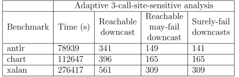
(37) Table 6.1: The DaCapo 2006 bench mark programs Benchmark Description parses grammar files, antlr then a parser and lexical analyzer is generated for each. uses JFreeChart to plot a number of complex line graphs chart and renders them as PDF. xalan transforms XML documents into HTML. 6.1. Size (MB) 0.619 2.1 1.2. Adaptivity vs. non-adaptivity. Firstly, Table 6.2 shows the results of the non-adaptive points-to analysis. Secondly, Table 6.3 shows the results of our adaptive points-to analysis. Here, the first column is the program name. The second column shows the runtime of the analysis. The column Reachble downcasts is the number of the reached downcasts. The fourth column is the number of downcast that may fail. In Table 6.2, there is only one column for the 3-callsite sensitive points-to analysis because this analysis is out of memory with all of the programs. In Table 6.3, the column Surely-fail downcasts is the number of downcasts that fail even if we run the analysis with the highest abstraction. In addition, we can prove whether a downcast surely fail at the highest abstraction by using the counterexample knowledge. Recall, our analysis uses partitioned repeated abstraction search. The “5partitioned 1-repeated” means the remaining downcasts are divided into group of five and the abstraction search is solved twice (one more time) in a single CEGAR iteration. In Table 6.3, for antlr, the number of surely fail downcasts is less than the number of may-fail downcasts because of the timeout of the MaxSAT solving step. Table 6.2 and Table 6.3 show that the number of reachable downcasts are the same for both the non analysis and our adaptive analysis. We remark that, in fact, the reachable downcasts coincide in the two analyses (i.e., not just the numbers). The tables show the followings: • Our adaptive 3-call-site-sensitive analysis do not do worse (equal or better) than the non-adaptive 2-call-site-sensitive analysis and of course it takes more time. • The non-adaptive 3-call-site-sensitive analysis does not finish. • The surely-fail downcast column shows that our method reaches the non-adaptive 3-call-site-sensitive analysis precision, except for antlr.. 6.2. Partition and repetition. I compare between the 0-repeated 5-partitioned abstraction search and the 1-repeated 5-partitioned search in Figure 6.1. I also compare between the 0-repeated 5-partitioned 31.

(38) Table 6.2: The results of the non-adaptive call-site-sensitive analysis 2-call-site-sensitive analysis Reachable Reachable may-fail Benchmark Time (s) downcasts downcasts antlr 21420 341 149 chart 24593 396 168 xalan 11994 561 313. 3-call-site-sensitive analysis. Out of memory Out of memory Out of memory. Table 6.3: The results of the adaptive (5-partitioned 1-repeated) points-to analysis Adaptive 3-call-site-sensitive analysis Reachable Reachable Surely-fail may-fail Benchmark Time (s) downcast downcasts downcast antlr 78939 341 149 141 chart 112647 396 165 165 xalan 276417 561 309 309. method and the 0-repeated 10-partitioned search in Figure 6.2. The graphs plot the number of downcasts that remain may-fail and detected to be surely-fail over the analysis run time. Both comparisons are on antlr. MF stands for may-fail downcasts and SF stands for surely-fail downcasts. The postfixes 5-0 and 5-1 respectively denote the 0-repetition and the 1-repetition with the 5-partition. Similarly, 10-0 stands for the 10-partitioned 0-repeated abstraction search. Basically, the 0-repetition is the analysis without the repeated abstraction search. Figure 6.1 shows that our repetition method is better than the non-repeated abstraction search with the antlr benchmark. The number of MF are decreased faster, while the SF are also proved quicker. In my experiment, the non-partitioned points-to analysis ends with timeout. Hence, our partitioned analysis is better than the non-partitioned analysis. In addition, the partitioned parameter k of the k-partitioned analysis is chosen by trial and error. Figure 6.2 shows that on the antlr benchmark the 5-partitioned analysis is better than the 10-partitioned one in proving sure-fail downcasts.. 32.

(39) 0-repetition vs. 1 -repetition on the Antlr benchmark 300. 250. No. Downcasts. 200. 150. 100. 50. 78969. 71877. 65495. 62339. 59302. 56899. 54480. 51942. 49408. 46834. 44114. 41295. 38767. 36080. 33375. 30501. 27598. 24573. 21579. 18616. 15833. 9737. 12837. 6416. 3059. 0. Time(s) MayFail-5-0 SureFail-5-0. MayFail-5-1 SureFail-5-1. Figure 6.1: 0-repetition vs. 1-repetition the antlr benchmark.. 5-partition vs. 10-partition on the anltr benchmark 300. No.Downcasts. 250. 200. 150. 100. 50. 2968 5938 8914 11870 14979 18616 21579 24573 27598 30203 33222 36080 38767 41295 44114 46834 49408 51942 54480 56899 59326 62339 65495 68704 71877 74648 77135 80038 83037 86018 89202 92728 96173. 0. Time(s) MayFail-5-0 SureFail-5-0. MayFail-10-0 SureFail-10-0. Figure 6.2: 5-partition vs. 10-partition on the antlr benchmark.. 33.