JAIST Repository: An Investigation of the Steven Eker's Approach to Associative-Commutative Matching [課題研究報告書]

(1)

Japan Advanced Institute of Science and Technology

JAIST Repository

https://dspace.jaist.ac.jp/

Title An Investigation of the Steven Eker's Approach to Associative-Commutative Matching [課題研究報告書] Author(s) Phan, Huu Tho

Citation

Issue Date 2018-03

Type Thesis or Dissertation Text version author

URL http://hdl.handle.net/10119/15197 Rights

Description Supervisor:緒方和博, 先端科学技術研究科, 修士

(2)

An Investigation of the Steven Eker’s Approach to

Associative-Commutative Matching

Phan Huu Tho

Graduate School of Advanced Science and Technology

Japan Advanced Institute of Science and Technology

(3)

Master’s Research Project Report

An Investigation of the Steven Eker’s Approach to

Associative-Commutative Matching

1610160 Phan Huu Tho

Supervisor : Kazuhiro Ogata

Main Examiner : Kazuhiro Ogata

Examiners : Kunihiko Hiraishi

Toshiaki Aoki

Nao Hirokawa

Graduate School of Advanced Science and Technology

Japan Advanced Institute of Science and Technology

Information Science

February, 2018

(4)

Abstract

This master’s project report focuses on the associative-commutative matching via bipar-tite graph matching including not only the basic approach but also the detailed algorithm to help other researchers get a better understanding about the algorithm created by S. M. Eker.

The problem we want to solve is the one consists of multiple terms where the subsets of functions symbols are associative-commutative. Eker’s approach to solving this com-plex problem is that we first change the form of both pattern term and subject term into ordered normal form because of the easier in representative and checking equality. Then making use of the recursive attribute of bipartite graph, we construct a hierarchy of bipartite graph matching problems containing AC subproblem and variable bindings. We try to find the variable bindings as soon as possible and concentrate on finding the variable clashes to backtrack rather than finding all possible solutions and then test them for consistency. From these graphs it can be found out the sets of solutions and build the semi-pure AC systems. When we solve the semi-pure AC system, we divide the variable into two type: the shared variable and owned variable with the different way of solving. Then, we try to find all the potential term in the subject terms to make the assignment to a variable. Afterwards, putting all the variable bindings and the solution from solving semi-pure AC system step to get the matching substitutions. This algorithm has imple-mented in Maude and showed the highest performance rewrite engine modulo AC. So we investigate in Eker’s approach to find the efficiency of his algorithm which can apply when we want to implement the independent software component.

Keywords: AC Matching Problem, Bipartite Graph Matching, Associativity, Commu-tativity, Ordered Normal Form, .

(5)

Acknowledgements

After almost two years working and studying with a lot of useful advice and various skilfully learning points, finally, I had been finished my thesis. I would first like to thank my supervisor, Professor Kazuhiro Ogata, you definitely supported and provided me with the most valuable directions both in research and my own life.

I also deeply appreciate my friends in Ogata lab, in JAIST for their full assistance to help me overcome the obstacle in my school life.

Finally, I want to spend the last meaningful word to my family, who always stand by me even if whatever happens to deliberate and give me your love unconditionally.

Thank you very much, everyone! Phan Huu Tho.

(6)

List of Figures

2.1 Rewriting process . . . 9

2.2 Examples of bipartite graph . . . 11

3.1 One level of an AC matching problem . . . 13

3.2 Decomposition of subproblem 1] . . . 14

3.3 Decomposition of subproblem 2 . . . 14

4.1 flattening a term . . . 20

4.2 Converting a flattened term to ordered normal form . . . 21

4.3 Building the match object . . . 22

4.4 Matching the non-AC skeleton . . . 23

4.5 Solving a graph hierarchy . . . 25

4.6 Solving an AC subproblem . . . 26

4.7 Sovling a bipartite graph problem . . . 27

4.8 Solving a system of semipure subproblem . . . 30

4.9 Finding an assignment to a shared variable . . . 31

4.10 Finding an assignment to an owned variable . . . 32

4.11 Selecting an assignment . . . 33

4.12 AC Matching algorithm . . . 34

4.13 Procedure build_match . . . 35

(8)

List of Tables

4.1 Data structure of graph hierarchy . . . 21 5.1 Running time of some examples with CafeOBJ and Maude (ms) . . . 36

(9)

Chapter 1 Introduction

Generally, Associative-Commutative (AC) pattern matching plays the important part in the world of functional programming, algebraic specification, verification as well as term rewriting systems which help to implement the functional programming languages, automated deduction [4] and hardware verification [6]. Term writing also can be viewed at both mechanizing equational logic and computing in the initial model of a set of equations [1].

Because of the limitation of pure term rewriting such as the associative and commutative axioms can be able to make the systems leading to the never-ending sequences of rewrites. To break down the condition of limited ability, one of the solution is that using congruence classes of terms instead of term themselves. One of the implementations of this approach is AC matching algorithm where AC is associative and commutative. The AC matching problem is known as an NP-complete, then S. M. Eker had presented the AC-matching algorithm [2] which runs productively on non-pathological problem instances. He had introduced the way to find ordered normal form then decompose the matching problem into the hierarchy of bipartite graphs. So solving these hierarchies get the matching substitution after combining with semi-pure AC problems.

1.1 Background and Motivation

Nowadays human being heavily relies on software systems which are existed in every single aspect of life. And it is inevitable that the modern software with cutting-edge technology has supported our lives much better and easier. Technologies systems then play the vital part in the development of mankind. This is undeniably the reason for increasing the growing awareness of making such systems highly reliable. Formal verification is one possible promising technique to make it possible to do so.

One formal verification technique is model checking that exhaustively traverses the reachable states of the state formalizing software systems. Associative-Commutative (AC) operators allow specifying state machines succinctly. To efficiently model check such succinctly specified state machine, it is necessary to make AC pattern matching efficiently.

(10)

1.2 Thesis Outline

This master project report will follow the below outline: Chapter 2: Preliminaries

This chapter shows the overview and some preliminaries to support for the main algorithms, AC pattern matching algorithm.

Chapter 3: The general approach

This chapter shows the basic algorithm with the concrete example to help the re-searcher understand the overview of Eker’s algorithm.

Chapter 4: Detailed description of algorithm

This chapter shows the implementation in pseudocode as detail as possible with the clear explanation.

Chapter 5: The significant efficiency of Eker’s algorithm

This chapter explains the reason why his algorithm so fast and such the techniques he used in his implementation.

Chapter 6: Conclusion and Future Work

This chapter shows the summary of our report and what we want to do in the near future.

(11)

Chapter 2 Preliminaries

In this chapter, we will describe some basic definitions to support the readers get fa-miliar with before moving to the main algorithm. It contains term writing, associative-commutative pattern matching, bipartite graph, Maude, and meta-programming.

2.1 Term rewriting

Term rewriting is a surprisingly simple computational paradigm that is based on the re-peated application of simplification rules. It is particularly suited for tasks like symbolic computation, program analysis, program transformation [3]. Understanding term rewrit-ing will help you to solve such tasks in a very effective manner, especially fully comprehend the whole content of Eker’s algorithm in this master research project.

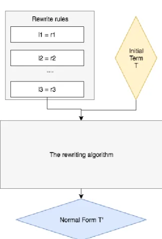
To apply the rewriting process in Figure 2.1 [3], we have to know several key words below:

• The initial term T is the term that needs to be simplified.

• The rewrite rules are the rules that will be applied in rewriting process

• The rewriting process will take one or more rewrite rules as the input and gradually reduced to a term that is cannot be simplified, then it is the output of the rewriting process and it is normal form T’.

The next term will be emphasized is that pattern match. Given a term t and a ground term s, the pattern match between t and s is the problem to decide whether there exists a substitution σ such that σ(t) = s. t may be called a pattern. If that is the case, s is called an instance of the pattern t and can match the pattern t with the substitution σ [5].

We want to introduce rewrite rules. A rewrite rule is a pair (l, r) of terms l and r such that the least sort of l is a sort of r, l is not a single variable, each variable occurring in r occurs in l. A term rewriting system (TRS) is a set of rewrite rules. [5].

The simple example of term rewriting is shown below:

(12)

Figure 2.1: Rewriting process

As can be seen from the above example, the initial term T is (7 − 5)2_{∗ (1 + 2), rewrite}

rules are the rules of elementary arithmetic, and the normal form T’ is 12. Normally, we will work with a term which is defined by the variable or function with zero or more terms. In that case, the complex hierarchy of term can be constructed.

2.2 Associative-Commutative (AC) Matching

There are some concepts we will work with: • Σ: Set of function symbols:

• χ: Set of variable symbols such as L, M, N,...

• Σ0: Set of constant symbols such as a, b, c, ... Note: Σ0 ⊂ Σ.

• ΣAC: Set of AC function symbols such as F, G, H,... Note: ΣAC ⊂ Σ.

• Σf ree: Set of free function symbols such as f, g, h,... Note: Σf ree ⊂ Σ.

• AC = {f (f (X, Y ), Z)) = f (X, f (Y, Z)), f (X, Y ) = f (Y, X)|f ∈ ΣAC}: Set of

(13)

The AC matching problem describes as: given a term p (the pattern term) and a term s (the subject term) we wish to find the substitutions σ such that AC ` pσ = s. These substitutions are called matching substitutions, and the problem to find the matching substitution is NP-complete, but a single solution can be found (if existing) in the polynomial time by transforming the problem into a graph matching problem if the pattern is restricted to being linear [2]. Via using this idea, we could able to apply into non-linear patterns and view the AC matching as a special case of AC unification.

When an AC matching problem can be written as p ≤?_AC s with the subject s containing no variables, then there are two more terms needed to comprehend are as follows:

• semi-pure problem: if p consists of a single AC function symbol with only variable symbol arguments.

• pure problem: if the subject s of the semi-pure problem consists of a single symbol with only constant symbol arguments.

2.3 Ordered Normal Form

The ordered normal form represents the equivalent relation agent for the congruence class by converting terms to ordered normal form so that we can easily check for equality modulo AC via syntactic equality. To deal with associative function symbols, we use the way that grouping associative operators to the right (or left). Then we can get the unique normal form via a multi-set of terms because the number of occurring of term is perhaps more than once. So ordered normal form can be viewed as the unique syntactic representation of multi-set of arguments when we use sorting and grouping inductively extended to terms.

To implement ordered normal form, first we will compare the top symbols of two terms. If it is different, the ordering on the term is defined by the ordering on their top symbols. On the other hand, if it holds the same top symbols, we will divide the type of function symbol into two cases: free function symbol and AC function symbol. Firstly, assuming that there are two terms with the same top symbol is free function. Then f (t1, ..., tn) >

f (u1, ..., un) if there is k ∈ {1, ..., n} such that tj = uj for j ∈ {1, ..., k − 1} and tk > uk.

Secondly, assuming that there are two terms with the same top symbol is AC function. Then F (tα1

1 , ..., tαnn) > F (u β1

1 , ..., uβmm) if there is k ∈ 1, ..., min(n, m) such that tj = uj and

αj = βj for j ∈ 1, ..., k − 1 and it holds one of the below conditions:

1. tk > uk; or

2. tk = uk and αk > βk; or

3. tk = uk and αk = βk and m = k and n > k.

After applying all these criterion, flattening nested AC function then sorting and grouping the AC function symbol, finally we get the ordered normal form. For examples:

(14)

• The ordered normal form of

F (F (a, F (c, F (g(a, b), g(a, c)))), F (b, F (b, F (g(b, a), g(c, b))))) is

F (a, b2, c, g(a, b), g(a, c), g(b, a), g(c, b)) • The ordered normal form of

G(G(G(a, G(a, G(a, b))), G(g(b, a), h(a))), h(b)) is

G(a3_{, b, g(b, a), h(a), h(b))}

F (F (F (F (a, a), F (b, F (a, b))), F (a, F (c, F (a, F (b, F (a, c)))))), a) is

F (a6_{, b}3_{, c}2₎

f (F (F (N, F (P, g(a, L))), F (N, g(M, b))),

G(G(G(U, a), G(h(Q), h(S))), G(G(g(T, a), N ), U )), V ) is

f (F (g(a, L), g(M, b), N2_{, P ), G(a, g(T, a), h(Q), h(S), N, U}2_{), V )} _.

2.4 Bipartite Graph

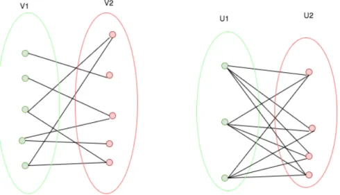
A bipartite graph, is also called bigraph, is a special graph which is its vertices set V can be divided into two disjoint subsets V = V1∪ V2, such that each edge connects a vertex

from one set to a vertex from another subset, in another word, it means every edge of graph has the e = (x, y) where x ∈ V1 and y ∈ V2. Remember that, there are no vertex

both in V1 or V2 are connected.

(15)

Chapter 3 The Basic Algorithm

Eker’s approach is not the easy idea to comprehend in a couple of minutes. That is the reason why I want to shows the basic approach first. In this part, the simple example will be introduced with step by step to support the researcher getting familiar with the solving path. Eker’s algorithm contains four steps:

1. Change the form of pattern term and subject term into ordered normal form 2. Decompose the matching problem into a hierarchy of bipartite graphs.

3. Solve the bipartite graph hierarchy and build a system of semi-pure AC problems. 4. Solve the system of semi-pure AC problems to get a matching substitution.

It can be seen that the first step is not complicated and be introduced in the previous chapter. In the second step, with the support from additional data, we can make the hierarchy of bipartite graphs from the matching problem. In the third step, it is necessary repeated to extract all the possible sets of solutions to the bipartite graph matching problem.

We will show all steps with the general explanation using the below example [2]: f (F (F (N, F (P, g(a, L))), F (N, g(M, b))),

G(G(G(U, a), G(h(Q), h(S))), G(G(g(T, a), N ), U )), V ) ≤?_AC f (F (F (a, F (c, F (g(a, b), g(a, c)))), F (b, F (b, F (g(b, a), g(c, b))))),

G(G(G(a, G(a, G(a, b))), G(g(b, a), h(a))), h(b)), F (a, b))

It is clear from the example that it is not easy to solve our example immediately because of consisting of many different and connected parts. Then the key idea is to divide the complex hard-to-solve problem (the original AC pattern matching) into the multiple easier-to-solve problems called AC semi-pure problem systems which we will deal with in step three and four.

3.1 Ordered Normal Form

In the previous chapter, we showed that it is able to flatten the terms involving associative and commutative functions symbols, then convert it to a normal form. It may produce

(16)

a new term with fewer characters. After these steps, sort and group term’s arguments will create the ordered normal form. Applying these methods in our problem, we get the ordered normal form as follow:

f (F (g(a, L), g(M, b), N2, P ), G(a, g(T, a), h(Q), h(S), N, U2), V ) ≤?_AC f (F (a, b2_{, g(a, b), g(a, c), g(b, a), g(c, b)), G(a}3_{, b, g(b, a), h(a), h(b)), F (a, b))}

3.2 Decomposition to bipartite graphs

From an overall perspective, it is very helpful and essential to get the knowledge of subterm or subproblem before describing bit by bit inherently recursive the way of decomposing to a bipartite graph of an AC matching problem. The definition of the level of a subterm within a term is the number of AC functions above it. And the definition of the level of a subproblem (p0, s0) within the whole AC matching problem (p, s) is the level of p0 within p.

Figure 3.1: One level of an AC matching problem

As is illustrated from the Figure 3.1, it highlights one level in the hierarchical decom-position of an AC matching problem with full components with some notices as follow: only one rectangle represents the further decomposition, the double rectangles reveals the possibly empty set of objects. Starting from the original AC matching problem which may contain the AC subproblem and the variable bindings, there is the first step to determine how many subproblems, how many variable bindings it has and keep in mind that it is also understandably conceivable. The way of determination of this issue is that confirm the type of pattern’s top symbol. If the non-AC top symbol is held by the pattern, it is called ”skeleton” and we treat them all the arguments which are under top symbol in order as the usual way. As the consequence of solving non-AC skeleton, the matching problem results in either the failure (if there is nothing match) or else leaving with a set of subproblem whose top symbols are AC and a set of variable bindings. There is a case that one or both of these sets are empty. Applying these principles to analyze our example, we get the set of variable bindings with single-member

V = F (a, b)

and the set of subproblems with AC top symbols containing the two members

F (g(a, L), g(M, b), N2, P ) ≤?_AC F (a, b2, g(a, b), g(a, c), g(b, a), g(c, b)) (1) G(a, g(T, a), h(Q), h(S), N, U2) ≤?_AC G(a3, b, g(b, a), h(a), h(b)) (2) If we find a variable clash (the same variable exists in the different bindings) then we have failure. When it comes to the decomposition of AC subproblems, we need to consider the arguments type directly under the AC top symbol as follows:

(17)

• constant in the pattern will be deleted from both pattern and subject term. After the deletion, there must be no constant in the pattern term. If there is any constant left in the pattern term, then there is a failure. Because we cannot match any constant in the pattern term to the subject term. Only variables and function symbols can be in the patter term after this step.

• function symbol (AC or free): for each function symbol ψ, we construct the bipartite graph containing pattern nodes (set of nodes) and subject nodes (set of nodes) under the same function ψ with the condition that the multiplicity of the pattern term must be lesser or equal to the multiplicity of the subject term, now the pair of subject node and pattern node is making the new problem with the same form as the original problem which can be recursively decomposed. If the pattern nodes have no corresponding subject node, there is a failure. In addition, if the subject node has no corresponding pattern node (e.i undeleted constants, terms headed by function symbols which is no graph), then it is called unmatched subject term.

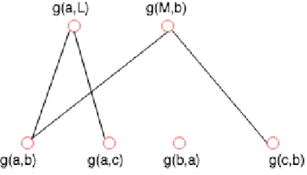
Figure 3.2: Decomposition of subproblem 1]

Figure 3.3: Decomposition of subproblem 2

Following these instructions and apply to our example, we can successfully decompose the subproblem 1, the subproblem 2 and show the result in Figure 3.2 and Figure 3.3 corresponding.

(18)

3.3 Solving the bipartite graph hierarchy

The goal of this step is to solve the bipartite graph hierarchy which consists of pattern nodes and subject nodes to make a system of semi-pure AC problems and the compatible set of solutions.

In term of finding an effective way to deal with bipartite graph matching problems, there is an answer that we can select each pattern node in turn and backtrack on failure. Whenever getting a successful solution by selecting an edge, all variable binding below and all graph problem can be solved when matching edge is found. By contrast, we conduct the backtracking or failure because of variable clashes. If variable clashes are found, it means the further path is not the solution, so we need to choose another path to solve by selecting another edge for this pair of pattern node and subject node. It also means that all the variable bindings while solving the bipartite matching problem with the wrong edge is not right anymore so that we need to retract. When finishing this step, if there is no failure, then the solution and a semi-pure AC problems are found.The semi-pure problems are constructed by the left AC problem in the left-hand side combining with unmatched subject subterm or any subject node left over from bipartite graph matching problem.

With regard to our example, in case of the decomposition of the subproblem 1, there are two pattern nodes and four nodes in subject side. As can be seen from the Figure 3.2, there are two edges from g(a, L) pattern node to g(a, b) and g(a, c). And there are two edges from g(M, b) pattern node to g(a, b) and g(c, b). No edge is connected to g(b, a) subject node, it means this node is surely added to the right hand side of semi-pure prob-lem afterwards. If we choose the first node from g(a, L) to g(a, b) to make an edge, then the next edge is chosen from g(M, b) must be to g(c, b) even if there is an edge between g(M, b) and g(a, b). The reason for this is that the multiplicity of both g(a, L) and g(a, b) are 1, after choosing an edge, we have to decrease the multiplicity from both nodes. So that we cannot make an edge between g(M, b) and g(a, b) anymore, if the multiplicity of subject node (g(a, b)) is greater than pattern node (g(a, L)), then there is a case, but in this case, there is no chance. All of pattern nodes is now chosen the edge already with leaving two subject nodes are g(a, c) and g(b, a) which will be added to semi-pure problem with unmatched subterms. From the first edge, we have the variable bindings hL, bi, and from the second edge, we have hM, ci. And the semi-pure problem consists N2 _{and P}

in the left hand side, a, b2_{, g(a, c) and g(b, a) in the right hand side. We have the first}

semi-pure problem as follow:

F (N2_{, P ) ≤}?

AC F (a, b2, g(a, c), g(b, a) .

With the same strategy, the two other choices of edges when an selected edge is from g(a, L) to g(a, c), the g(M, b) pattern node can connect to g(a, b) or g(c, b). It results two other sets of variable bindings and semi-pure problems as follow:

{hL, ci, hM, ai}, F (N2_{, P ) ≤}?

AC F (a, b2, g(b, a), g(c, b))

{hL, ci, hM, ci}, F (N2_{, P ) ≤}?

AC F (a, b2, g(a, b), g(b, a))

In terms of the composition of the subproblem 2 applying the previous rule, it results two sets of variable bindings and semi-pure problem as follow:

{hT, bi, hQ, ai hS, bi}, G(N, U2_{) ≤}?

(19)

{hT, bi, hQ, bi hS, ai}, G(N, U2_{) ≤}?

AC G(a2, b)

Thanks to the results of decomposition of subproblem 1 with three semi-pure problems and subproblem 2 with two semi-pure problems, we can build totally 3 × 2 = 6 possible semi-pure AC systems.

3.4 Solving the semi-pure AC system

In the fourth step, it will be repeated in order to extract all matching substitutions from the semi-pure AC system which is the result of step three. We will consider the solution under three cases below.

Firstly, we will show the solution in general point of views. The easiest systems are that it consists of an only single semi-pure AC problem. Therefore, if we replace the term headed by AC top symbol on the right-hand side by the fresh constants then the semi-pure AC problem will be considered as the pure AC problem following by:

F (Xα1 1 , ..., X αn n ) ≤ ? AC F (c β1 1 , ..., c βm m )

Keep in mind that each variable can be assigned to one or more constants, if more than one constant are assigned to one variable, then all the assigned constants will be treated as the arguments under AC top symbol. Because the multiplicity of the left-hand side must be equal to the right-hand side in any case, so that the solution must satisfy the below Diophantine:    α1x1,1 + . . . + αnxn,1 = β1 .. . ... ... α1x1,m + . . . + αnxn,m = βm   

Condition for all variables with i ∈ {1, ..., n} because every variables must be assigned to something:

m

X

j=1

xi,j ≥ 1.

Secondly, another striking feature is that the consists of k semi-pure AC problem in semi-pure AC systems occur, then we will get the same Diophantine formulation with k × m equations.

Lastly, the most complicated case, the semi-pure AC system contains many semi-pure problems with different AC top symbols. In this case, the beginning hypothesis about a replacement of term cannot work anymore. It means the variables occur under at least two AC semi-pure problem with different AC top symbol must be assigned to only one term. If not, there is a failure unless one of the arguments on the right-hand side of one semi-pure AC problem has as its head the AC top symbol of another semi-pure AC problem. Here is the example of the exception.

(20)

G(L, N ) ≤?_AC G(F (a, b), c, d)

As can be seen from the semi-pure AC system, both a and b can be assigned to L in the first semi-pure AC problem, then it means L = F (a, b) because F is the top function symbol of the first problem. One more thing is that in the second problem, the term F (a, b) occurs in the right hand side under G top symbol. So it is possibly a solution for our assignment. After all, we have to matching substitution below.

L = F (a, b), M = c, N = G(c, d)

Another needed step to make clear should be that we divide the type of variable into two classes: owned variable and shared variable. The owned variable is the variable occurring under only single function symbol. And shared variable is the variable occurring under two or more different function symbol. Whenever the assignment is made, the multiplicities of the related terms must be reduced, and the procedure will continuously conduct to find a solution or facing the failure.

As we know that we have 6 possible semi-pure AC systems with the same solving path. So we take the first system into our consideration as follow:

F (N2, P ) ≤?_AC F (a, b2, g(a, c), g(b, a)) G(N, U2_{) ≤}?

AC G(a2, b)

The type of variables: • Shared variable: N

• Owned variable under F is P , owned variable under G is U Then we can show the above system in the tabular form:

N P U a b g(a, c) g(b, a)

F 2 1 0 1 2 1 1

G 1 0 2 2 1 0 0

It is obviously clear from the tabular form that N is assigned to b because N is the shared variable, it means the multiplicity of N has to satisfy both in F and G function, if not, there is a failure. So that b is the only choice of N in this case. Then we have a new tabular form:

N P U a b g(a, c) g(b, a)

F 0 1 0 1 0 1 1

G 0 0 2 2 0 0 0

Combining with the variable bindings from the previous steps, we get the matching substitution for the first semi-pure AC system:

L = b M = c N = b P = F (a, g(a, c), g(b, a)) Q = a A = b T = b U = a

(21)

Chapter 4 Detailed Description of Algorithm

This chapter supports the basic algorithm via giving the information about all steps with pseudocode and explain comprehensively.

From a general perspective, the data structure of hierarchy of bipartite graph is recursive which is demonstrated by the form of a problem under edge between pattern node and a subject node is the same form with original AC matching problem. Consequently, it leads to using recursion for traversing bipartite graph rather than search space. In the solving procedure, we wish to find one solution first then based on the previous solution to figure out the next solution. If not, there is a failure, then we backtrack to an original matching problem to discover another solution. As we know, the recursive procedure costs a lot of time and effort. To limit this weak point, we only use recursive for traversing data structure itself. In another part it is needed to be done with non-recursive way, we use stack frame for the calling procedure (caller) and it is accessible by the direct route.

4.1 Notational considerations

Because of the complexity of Eker’s algorithm, to explain and make it intelligible and comprehensible, we highlight the pseudocode and standard mathematical notation with some supported notation which will be defined below.

Firstly, we want to use the presupposition that there is a top_symbol function of a term such that top_symbol(t) is the outermost function symbol of term t, or t itself if t is a constant or a variable. The nil value is also used to emphasize the empty set or no return value. When it comes to an assignment, we want to distinguish between the symbol 0 :=0 and 0 ⇐0_{. The former stands for assignments to temporary and the latter}

stands for destructively update part of a complicated data structure.

Secondly, to make the intricate structures look more friendly, there are some container data types that it would be helpful:

• tuples/records: it is the same usual meaning as tuple notation in mathematical field, now we also use it to form the object, contain the ordered list of elements. Examples: h = hA, Bi, b = hx, ti, tm = ht, αi.

(22)

• sets: the unordered list of unique elements, the same meaning in its usual notation. Example: {a, b, c}

• multisets: the same meaning with set except allowing duplicated elements. Notice that the set is also multiset. Example: {a, a, b}

• stacks: the collection of elements containing two principle operation which are push and pop to add and remove the element.

• arrays: the container of elements with index which is can accessible by using a[i] notation with index i.

Last but not least, there are some supported operations which use to traverse our data types:

• first(s): return the first element in s. • last(s): return the last element in s.

• next(s,e): return the element following e in s. • previous(s,e): return the element preceding e in s.

4.2 Conversion to ordered normal form

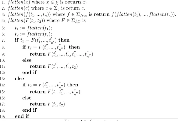
The first step of converting to ordered normal form is flatten the term using the algorithm illustrated in Figure 4.1 [2].

It is clear from the pseudocode for flattering a term that there are four cases depending on the type of terms. If the term’s type is

• constant or variable, then return the constant or variable itself respectively.

• free function, then return the flattening of each argument under free function recur-sively.

• AC function, then there are a little more complicated. First we need to flatten two arguments as t1 and t2 under AC function symbol. After that, both of arguments

have the same top symbol with the original term, then it obviously combines all the under t1 and t2 to under the original term’s top symbol after removing the top

symbol of t1 and t2. If one of argument holds the different top symbol with the

original top symbol, the combining the different term itself with all argument of the other term under the top symbol of the original term. Otherwise, just keep the t1

and t2 itself under the top function symbol.

After flattening all the terms, we continuously sort the argument list of AC operators and combine identical subterms which show in details in Figure 4.2 [2]. If the type of term is

(23)

1: f latten(x) where x ∈ χ is return x. 2: f latten(c) where c ∈ Σ0 is return c.

3: f latten(f (t1, ..., tn)) where f ∈ Σf ree is return f (f latten(t1), ..., f latten(tn)).

4: f latten(F (t1, t2)) where F ∈ ΣAC is 5: t1 := f latten(t1); 6: t2 := f latten(t2); 7: if t1 = F (t 0 1, ..., t 0 n0) then 8: if t2 = F (t 00 1, ..., t 00 n00) then 9: return F (t0₁, ..., t0_n, t00₁, ..., t00 n00) 10: else 11: return F (t0₁, ..., t0_n, t2) 12: end if 13: else 14: if t2 = F (t 00 1, ..., t 00 n00) then 15: return F (t1, t 00 1, ..., t 00 n00) 16: else 17: return F (t1, t2) 18: end if 19: end if

Figure 4.1: flattening a term

• constant or variable, then return the constant or variable itself in order given. • free function, then return the ordered normal form of each argument under free

function recursively such as f (onf (t1), ..., onf (tn)).

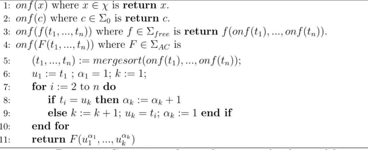
• AC function onf (F (t1, ..., tn)), then the first step is that make the ordered normal

form of all arguments under the AC function from onf (t1) to onf (tn), then sort the

argument list of AC operators using merge sort as (t1, ..., tn) := mergesort(onf (t1), ..., onf (tn)).

Then we try to group the same subterm together to make the term shorter by in-creasing the multiplicity of subterms.

4.3 Building the graph hierarchy

4.3.1 The graph hierarchy data structure

From now on, we assume that all terms have been transferred into ordered normal form. And basically the graph hierarchy data structure looks like the Figure 3.1 [2] which had shown in the last chapter. In details, it will be described in the Table 4.1.

(24)

1: onf (x) where x ∈ χ is return x. 2: onf (c) where c ∈ Σ0 is return c.

3: onf (f (t1, ..., tn)) where f ∈ Σf ree is return f (onf (t1), ..., onf (tn)).

4: onf (F (t1, ..., tn)) where F ∈ ΣAC is 5: (t1, ..., tn) := mergesort(onf (t1), ..., onf (tn)); 6: u1 := t1 ; α1 = 1; k := 1; 7: for i := 2 to n do 8: if ti = uk then αk := αk+ 1 9: else k := k + 1; uk = ti; αk := 1 end if 10: end for 11: return F (uα1 1 , ..., u αk k )

Figure 4.2: Converting a flattened term to ordered normal form

Name Notation Explanation

Graph hierarchy: h h = hA, Bi A = h.ac_subproblems: a set of AC subproblem B = h.bindings: a set of variable bindings Variable bindings: b b = hx, ti x = b.variable: a variable

t = b.term: a term

AC subproblem: a a = hf, V, L, Gi

f = a.top_symbol: an AC symbol function V = a.variables: a set of term-multiplicity pairs

where all term are variable

L = a.lef tovers: a set of term-multiplicity pairs G = a.graphs: set of bipartite graph problem Term-multiplicity

pair: tm tm = ht, αi

t = tm.term: a term

α = tm.multiplicity: a positive integer Biparte graph

problem: g g = hf, P, Si

f = g.top_symbol: a function symbol P = g.pattern_nodes: a set of pattern nodes S = g.subject_nodes: a set of term multiplicity-pairs

Pattern node: pn pn = hp, α, E, ci

p = pn.term: a term

α = pn.multiplicity: a positive integer E = pn.edges: a set of edges

c = pn.current_edge: an edge drawn from E, used to traverse graph hierarchy and hold the current state with initial value being nil Edge: e e = hs, hi

s = e.subject: a term such that for some β hs, βi is an element of g.subject_nodes

h = e.consequences: a graph hierarchy Table 4.1: Data structure of graph hierarchy

(25)

4.3.2 The construction algorithm

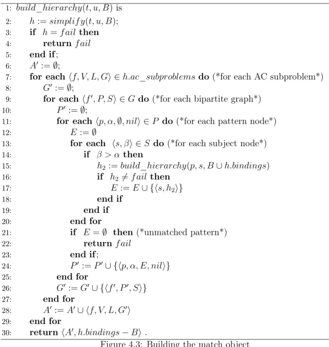
1: build_hierarchy(t, u, B) is 2: h := simplif y(t, u, B); 3: if h = f ail then 4: return f ail 5: end if ; 6: A0 := ∅;

7: for each hf, V, L, Gi ∈ h.ac_subproblems do (*for each AC subproblem*) 8: G0 := ∅;

9: for each hf0, P, Si ∈ G do (*for each bipartite graph*) 10: P0 := ∅;

11: for each hp, α, ∅, nili ∈ P do (*for each pattern node*)

12: E := ∅

13: for each hs, βi ∈ S do (*for each subject node*)

14: if β > α then 15: h2 := build_hierarchy(p, s, B ∪ h.bindings) 16: if h2 6= f ail then 17: E := E ∪ {hs, h2i} 18: end if 19: end if 20: end for

21: if E = ∅ then (*unmatched pattern*)

22: return f ail 23: end if ; 24: P0 := P0 ∪ {hp, α, E, nili} 25: end for 26: G0 := G0∪ {hf0_{, P}0_{, Si}} 27: end for 28: A0 := A0∪ hf, V, L, G0_i 29: end for 30: return hA0, h.bindings − Bi .

Figure 4.3: Building the match object

In the first period, the build_hierarchy procedure represented in Figure 4.3 [2] takes a pattern term p, a subject term s, and an initially empty set of variable bindings B as its arguments in order to generate all level of hierarchy of bipartite graph and construct their data structure. The first command it does is to call the simplif y procedure shown in Figure 4.4 [2] via h := simplif y(t, u, B). The output of simplif ies procedure is either f ail if the variable clashes are found and there is no possible match or the single level of graph hierarchy with empty edge sets. The purpose of simplif y function is to recursively traverse in the topmost level of the pattern term, the subject term, then try to match

(26)

1: simplif y(x, t, B) where x ∈ χ is

2: if (∃hx0, t0i ∈ B).[x0 _{= x ∧ t}0 _{6= t] then return f ail else return h∅, {(x, t)}i}

3: end if

4: simplif y(c, t, B) where c ∈ Σ0 is

5: if c = t then return h∅, ∅i else return f ail end if 6: simplif y(f (p1, ..., pn), t, B) where f ∈ Σf ree is

7: if t = f (s1, ..., sn) then 8: A := ∅ 9: for i := 1 to n do 10: h := simplif y(pi, si, B); 11: if h = f ail then 12: return f ail 13: end if

14: B := B ∪ h.bindings; (*collect bindings*)

15: A := A ∪ h.ac_subproblems (*collect AC subproblems*) 16: end for 17: return hA, Bi 18: else 19: return f ail 20: end if 21: simplif y(F (pα1 1 , ..., pαnn), t, B) where F ∈ ΣAC is 22: if t = F (sβ1 1 , ..., sβmm) then

23: V := {hpi, αii|pi ∈ χ}; (*collect pattern variables*)

24: for each i such that pi ∈ Σ0 do (*eliminate pattern constants*)

25: if (∃j).[sj = pi∧ βj ≥ αi] then βj := βj− αi else return f ail end if

26: end for 27: G := ∅

28: for each f ∈ Σ − Σ0 such that (∃i).[topsymbol(pi) = f ] do (*build bipartite

graphs*)

29: P := {hpj, αj, ∅, nili|topsymbol(pj) = f }; (*pattern nodes*)

30: S := {hsj, βji|topsymbol(sj) = f }; (*subject nodes*)

31: G := G ∪ {hf, P, Si} (*add bipartite graph with no edges*) 32: end for

33: L := {hsi, βii|(∀hf, P, Si ∈ G).[top_symbol(si) 6= f ]∧βi > 0}; (*collect leftover

subject terms*)

34: return h{hF, V, L, Gi}, ∅i

35: else

36: return f ail 37: end if

(27)

function symbols, variables, and constants. The input of simplif y function is the same as the parameters of build_hierarchy function as (x, t, B), x is the pattern term, t is the subject term, and B is the variable bindings from build_hierarchy procedure.

Firstly, if the pattern term x is variable, then we look for the variable bindings in B to find the existing of variable clashes comparing with hx, ti. If any, return f ail, if not, return the graph hierarchy with an empty set of subproblem and set of variable binding containing single item {hx, ti}.

Secondly, if the pattern term x is constant such as c, then if c is the same value with subject term t, then return empty of graph hierarchy h∅, ∅i. Otherwise, it returns f ail because of nor existing of variable binding neither graph hierarchy.

Thirdly, in case the pattern term is the term with free function symbol as the top function formed f (p1, ..., pn), if the subject term t is not the term with free function f ,

then return obviously f ail. There is no chance of finding a matching. On the other hand, if the subject term t holds the top symbol as the free function such as f (s1, ..., sn),

then for each pair parameters pi and si combining with B, creating an empty set of AC

subproblem A, we recursively operate the function simplif y(pi, si, B). Then, we collect

all the variable bindings into B and AC subproblems into A. After all, we return the bigraph hierarchy hA, Bi.

Lastly, if the pattern term is under AC function symbol as simplif y(F (pα1

1 , ..., pαnn), t, B).

So that the subject term must be the same form as the pattern term with F as the AC function symbol unless it returns f ail. The first move is that we collect the pattern variable containing multiplicity which is stored in set V . Then, it is needed to eliminate pattern constant by comparing constant between pattern terms and subject terms and decrementing the multiplicity with the term duplication. Then, for each pair of pattern subterms and subject subterms, at that time we build the bipartite graph G with no edge from pattern subterms as the pattern nodes P and subject subterms as the subject nodes S. Next, we collect the leftover subject term L. The last step is to return hF, V, L, Gi with an empty variable binding set.

4.4 Solving the graph matching problems

The answer of finding all the substitutions for the root AC matching problem is extremely complicated. One of the possible solving paths, as we know, is to divide the original pattern matching into the multiple levels of bipartite graph called graph hierarchy. The problem is solving the whole graph hierarchy is actually not easy. So that we come up with solving the single bipartite graph matching problem g = hf, P, Si is the temporary step forward to the final solution. And the result of bipartite graph problem is called a localsolution which is the assignment between the pattern node in P and the subject node in S with two required conditions [2]:

1. The subject node sn is assigned to pn is the target of one of the edges in pn (recall that edges are associated with each pattern node rather than the graph).

(28)

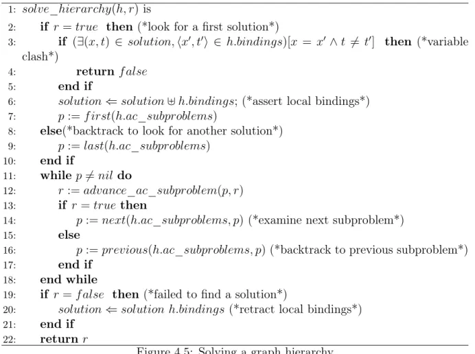
1: solve_hierarchy(h, r) is

2: if r = true then (*look for a first solution*)

3: if (∃(x, t) ∈ solution, hx0, t0i ∈ h.bindings)[x = x0 _{∧ t 6= t}0_{] then (*variable}

clash*)

4: return f alse 5: end if

6: solution ⇐ solution ] h.bindings; (*assert local bindings*) 7: p := f irst(h.ac_subproblems)

8: else(*backtrack to look for another solution*) 9: p := last(h.ac_subproblems)

10: end if

11: while p 6= nil do

12: r := advance_ac_subproblem(p, r) 13: if r = true then

14: p := next(h.ac_subproblems, p) (*examine next subproblem*)

15: else

16: p := previous(h.ac_subproblems, p) (*backtrack to previous subproblem*) 17: end if

18: end while

19: if r = f alse then (*failed to find a solution*)

20: solution ⇐ solution h.bindings (*retract local bindings*) 21: end if

22: return r

Figure 4.5: Solving a graph hierarchy

2. The sum of the multiplicities of all of the pattern nodes to which sn is assigned is less or equal to the multiplicity of sn.

From the condition 1, we understand that we need to keep track of the set of pattern nodes. Then fixing the chosen edge from pattern node to subject node is to create the possible smaller graph hierarchy with its local solution (may be null) and recursively search through the graph hierarchy, after that we can still keep the pattern node and change the subject node to create a new possible graph hierarchy until all elements in set of pattern nodes and set of subject nodes have been traversed. The most bottom level and of the graph hierarchy is the graph hierarchy containing no bipartite graph problem which is able to solved easily without serious issues. Contrastly, we have to define the local solution of the graph problem through the consequence of all the bottom level of the graph problem’s solution of its hierarchies, then the solution is the union set of these consequence sets.

Before going to the further step, we need to know how to solve the simplest graph hier-archy h = hA, Bi containing no bipartite graph problem. A is the set of AC subproblem which A’s element is ai = hf, V, L, ∅i ∈ A (i = 0 → n, n is the number of AC subproblem

(29)

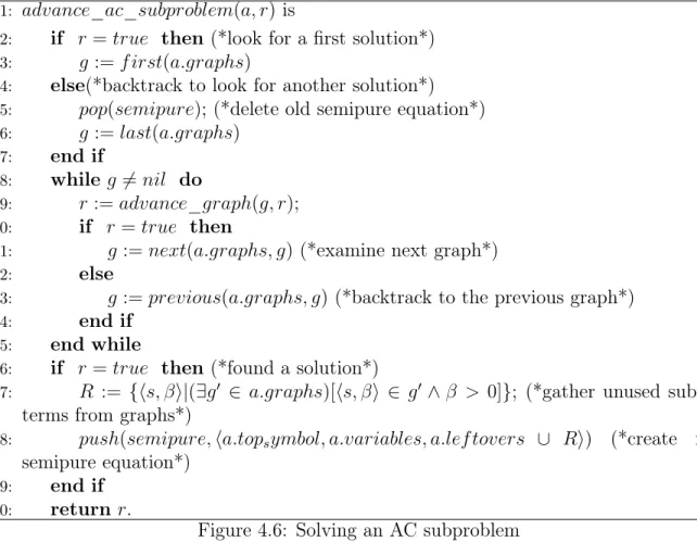
1: advance_ac_subproblem(a, r) is

2: if r = true then (*look for a first solution*) 3: g := f irst(a.graphs)

4: else(*backtrack to look for another solution*) 5: pop(semipure); (*delete old semipure equation*) 6: g := last(a.graphs)

7: end if

8: while g 6= nil do

9: r := advance_graph(g, r); 10: if r = true then

11: g := next(a.graphs, g) (*examine next graph*)

12: else

13: g := previous(a.graphs, g) (*backtrack to the previous graph*) 14: end if

15: end while

16: if r = true then (*found a solution*)

17: R := {hs, βi|(∃g0 ∈ a.graphs)[hs, βi ∈ g0 _{∧ β > 0]}; (*gather unused subject}

terms from graphs*)

18: push(semipure, ha.topsymbol, a.variables, a.lef tovers ∪ Ri) (*create new

semipure equation*) 19: end if

20: return r.

Figure 4.6: Solving an AC subproblem

function, V as arguments in the left-hand side and L as the arguments in the right-hand side. From those semi-pure problem combining with variable bindings B, we have the solution of graph hierarchy h. For the more complex graph hierarchy which is including bipartite graph problem, we need to define recursively that each edge of bipartite graph is the lower level of graph hierarchy until the top bottom level to reach the simplest graph hierarchy which contains no bipartite graph, and the variable bindings B is the union of all variable bindings in each graph hierarchies which is always consistent, it means that for the same variable, it musts be assigned to the same term in whole variable bindings.

For the implementation of solving hierarchy, we use solve_hierarchy(h, r) procedure which h is the graph hierarchy, r is the flag whose value is true if we are looking for further step of the first solution, f alse if we change the direction of finding another so-lution. Inside the procedure solve_hierarchy(h, r), we call the sub procedure named advace_ac_subproblem(a, r) with AC subproblem as the first argument and flag as the second argument. Then, as the inner part of advace_ac_subproblem(a, r), we call advace_graph(g, r) with a graph as the first argument and the second argument is the flag r coming from a super procedure. These three recursive procedures will traverse all the level of the hierarchy to create the variable bindings called solution and a stack of semipure problems which having the semi-pure AC problems from solving these bipartite

(30)

1: advance_graph(g, r) is

2: if r = true then (*look for a first solution*) 3: pn := f irst(g.pattern_nodes)

4: else(*backtrack to look for another solution*) 5: pn := last(g.pattern_nodes)

6: end if

7: while pn 6= nil do

8: if r = true then (*look for a first match*) 9: e := f irst(pn.edges)

10: r := f alse (*initially we have no match*)

11: else(*see if current match can be solved in a new way*) 12: e := pn.current_edge;

13: if solve_hierarchy(e.consequences, f lase) = true then 14: r := true (*current match is still good*)

15: else(*look for another match*)

16: sn := hs, βi ∈ g.subject_nodes such that s = e.subject;

17: (*destructively update g.subject_nodes through this reference*) 18: sn.multiplicity ⇐ sn.multiplicity + pn.multiplicity; (*restore old

sub-ject’s multiplicity*)

19: e := next(pn.edge, e)

20: end if

21: end if

22: while r = f alse ∧ e 6= nil do

23: sn := hs, βi ∈ g.subject_nodes such that s = e.subject;

24: (*destructively update g.subject_nodes through this reference*)

25: if sn.multiplicity ≥ pn.multiplicity ∧

solve_hierarchy(e.consequence, true) = true then 26: pn.current_edge ⇐ e;

27: sn.multiplicity ⇐ sn.multiplicity − pn.multiplicity; 28: r := true (*we have a successful match*)

29: else

30: e := next(pn.edges, e)

31: end if

32: end while

33: if r = true then (*we found a match - advance to next pattern node*) 34: pn := next(g.pattern_nodes, pn)

35: else(*we did not find a match - backtrack to previous pattern node*) 36: pn := previous(g.pattern_nodes, pn)

37: end if 38: end while 39: return r.

(31)

graphs. The main idea of figuring out the solution is that we try to find the first solution with testing the variable clashes continuously and update destructively the solution, if at any time we occur the variable clashes, we change the direction to find another solution. The first procedure is solve_hierarchy(h, r) described in Figure 4.5 [2] aiming to solve the graph hierarchy h. The first step is checking flag r, it means looking for a first solution. If flag is true, we continuously check the variable clashes in h.bindings, if found, return f alse immediately. If not, we do destructively update the global multiset of bindings solution with h.bindings. Then we traverse the first AC subproblem. If the flag is f alse, we traverse the last AC subproblem. The next step is dealing with AC subproblems in a loop, for each AC subproblem, it will call advance_ac_subproblem to operate and return the value to flag r. Appling the unified strategy, we will try with the next AC subproblem if the flag is true, if not, backtrack to the previous AC subproblem. After all, if the flag is f alse, it means that we need to retract the local bindings by substracting the h.bindings in the global solution set, then destructively update solution.

The second procedure is advance_ac_subproblem highlighted in Figure 4.6 [2] to solve the AC subproblem obviously. The first step is checking flag r, we will look for the first solution by solving the first graph in a.graphs set. If not, we backtrack to look for another solution through deleting the top the old semi-pure equation traversing the last graph in a.graphs set. The second step is the loop calling advance_graph to solve all the graphs one by one. If the result of advance_graph procedure returns true, we will examine next graph, if not, we backtrack to the previous graph. After traversing all graphs, if the flag is still true, we will gather the unused subject terms from graphs and create the new semi-pure equation which contains the top symbol, the variable, the leftover and the unused subject terms from graphs.

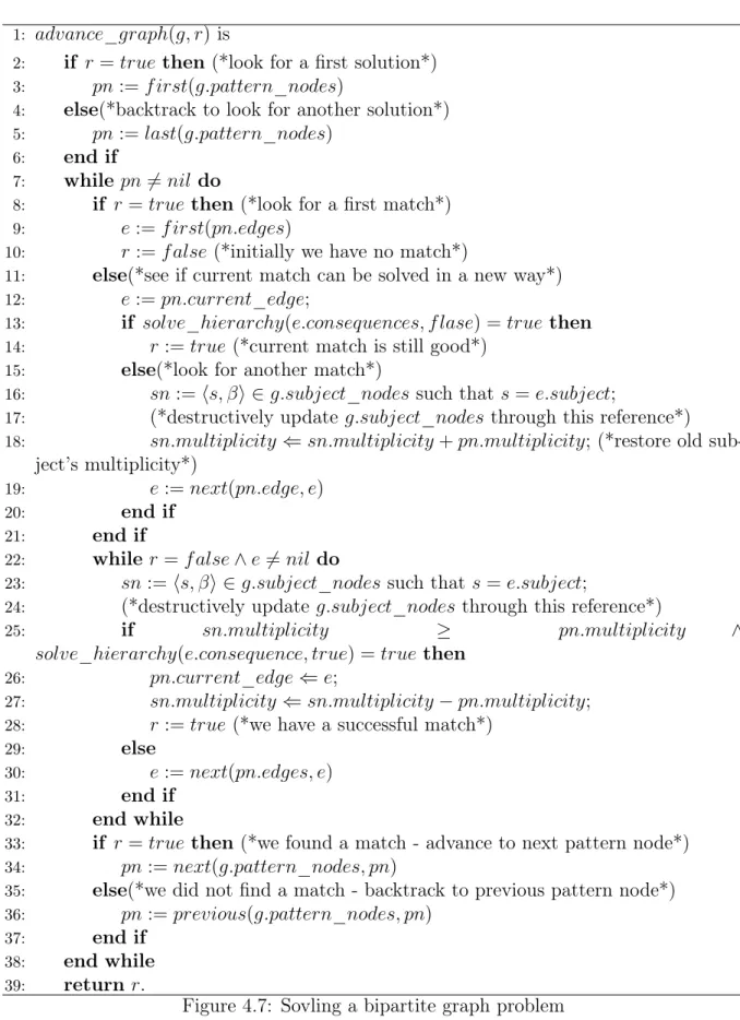
The last procedure is advancegraph shown in Figure 4.7 [2] which solves the bipartite

graph problem via choosing the suitable edge between a pattern node one by one and a set of subject nodes. The first step is depending on the value of the flag, if it is true, we look for the first solution, if not, backtrack to look for another solution by changing the pattern node from the first of element into the last element in pattern nodes set. The next step is to find the lower graph hierarchy by choosing an edge. We continuously check the flag, if it is f alse, we have to solve the matching edge in a new way by calling again procedure solve_hierarchy with current edges being the graph hierarchy as the first argument and the f alse flag as the second argument. If the result returns true, it means the current match is still good. If not, we need to destructively update set of subject nodes, restore old subject’s multiplicity and choose the next edge to search again. Then, we go to loop to find the suitable current edge while the flag is f alse and the current edge is not null. We check whether the multiplicity of a subject node is greater than the multiplicity of pattern node and the result of solve_hierarchy of current edge with flag true still return true. Hence we update the current edge, subtract the multiplicity of the subject node by the multiplicity of pattern node and reset the value of the flag is true because of a new successful match found. Otherwise, we choose another pattern node to solve. After all, if we find the match, we continue with the next pattern node, if not, we backtrack to the previous node.

(32)

Overall, because of the finite of the root graph hierarchy, we finally possibly can put an end to this recursive procedure. The first case is that there is no consistent solution and return false. By contrast, we have the multiset solution containing the variable bindings and the stack semipure containing the semi-pure AC problems associated with a consistent solution of h.

4.5 Rebuilding the semi-pure AC system

For the better efficiency, we will rebuild the semi-pure AC system which is the result of solving the graph matching problem step. We transform the semi-pure system into a tuple s = hV, T, Ei whose are:

• s.variable = V : a set of variable-records which is v = hi, o, sa, ms, ma, cs, cai ∈ V – v.index = i: the index unique of the variable

– v.owner = o: if v is the owned variable, v.owner = shared: if v is the shared variable.

– v.singleassigment = sa: a term index for the assignment of variable v

– v.max_size = ms: an integer, the maximum assignment size to variable v – v.current_size = cs: an integer, the current assignment size to variable v – v.max_assign = ma: an arrays of integers indexed by term indices. – v.current_assign = ca: an arrays of integers indexed by term indices. • s.terms = T : a set of term-record which is t = hi, Ii

– t.index = i: an index unique to the term

– t.subterm_indices = I: a set of index-multiplicity pairs for the subterms of the term. (if the term is headed by AC function symbol and the subterm is not under as the right hand side term, so that the value of t.subterm_indices is ∅)

• s.equations = E: a set of equation-records which is e = hf, vm, tmi ∈ E. – e.top_symbol = f : an AC function symbol

– e.variable_multiplicity: an array of integers indexed by variable indices. – e.term_multiplicity: an array of integer indexed by term indices.

4.6 Solving the semi-pure AC system

From an overall perspective, the solving the semi-pure system containing six procedures to find the possible assignments of variables. We also keep the strategy that applied in

(33)

the previous procedures that taking the flag r for the direction, r = true if we want to find to the first solution, r = f alse if we want to find another solution. And the result of flag r also respect the output of our problem, r = true if we found the solution, if not, we did not find the solution.

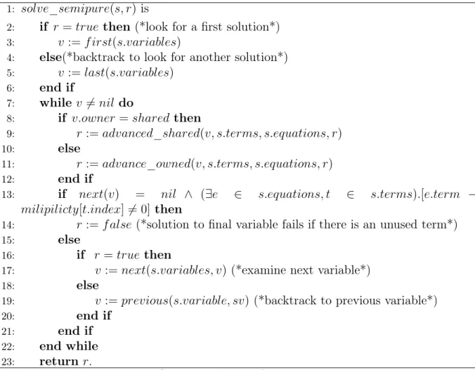
The first procedure is solve_semipure shown in Figure 4.8 [2] which the most important procedure and it will call the remaining procedure inside itself. Then, as we mentioned before, it will check the flag for the direction, we will look for a first solution if the flag is true, then try to find the assignment of the first variable, if not, we will backtrack to look for another solution, then try to find the assignment of the last variable. After that, we need to check whether the chosen variable is the owned variable or the shared variable to call the suitable procedure for each type of variable. After assignment for all the variables, if there are any unused term that is not be assigned to any variable, it means that the solution to a final variable is not suitable, then set the flag to f alse for a return value. If there is no unused term is available, we continuously check the return value of the flag, if it is true, we will examine the next variable, if not, we do the backtrack to the previous variable. We will repeat this loop until the last variable.

1: solve_semipure(s, r) is

2: if r = true then (*look for a first solution*) 3: v := f irst(s.variables)

4: else(*backtrack to look for another solution*) 5: v := last(s.variables)

6: end if

7: while v 6= nil do

8: if v.owner = shared then

9: r := advanced_shared(v, s.terms, s.equations, r)

10: else

11: r := advance_owned(v, s.terms, s.equations, r) 12: end if

13: if next(v) = nil ∧ (∃e ∈ s.equations, t ∈ s.terms).[e.term − milipilicty[t.index] 6= 0] then

14: r := f alse (*solution to final variable fails if there is an unused term*)

15: else

16: if r = true then

17: v := next(s.variables, v) (*examine next variable*)

18: else

19: v := previous(s.variable, sv) (*backtrack to previous variable*)

20: end if

21: end if 22: end while 23: return r.

(34)

1: advance_shared(v, T, E, r) is

2: if r = true then (*look for a first assignment*) 3: t := f irst(T )

4: else(*backtrack to look for another assignment*)

5: updateshared(v, v.singleassignment, E, 1);(*replace subject terms used up by

previous assignment*) 6: t := next(v.singleassignment) 7: end if 8: while t 6= nil do 9: for each e ∈ E do 10: vm := e.variable_multiplicity[v.index]; 11: if vm > 0 then

12: if t.top_symbol = e.top_symbol then

13: if t.subterm_indices = ∅ ∨ (∃hi, mi ∈

t.subterm_indices).[e.term_multiplicity[i] < m × vm] then

14: goto f ailure

15: end if

16: else

17: if e.term_multiplicity[t.index] < vm then goto f ailure

18: end if

19: end if

20: end if

21: end for

22: v.single_assignment ⇐ t;

23: update_shared(v, t, E, −1); (*remove used up subject terms*) 24: return true;

25: f ailure:

26: t = next(T, t) (*try next term*) 27: end while

28: return f alse.

29: update_shared(v, t, E, n) is 30: for each e ∈ E do

31: if t.top_symbol = e.top_symbol then 32: for each hi, mi ∈ t.subterm_indices do

33: e.term_multiplicity[i] ⇐ e.term_multiplicity[i] + n × m × e.variable_multiplicity[v.index] 34: end for 35: else 36: e.term_multiplicity[t.index] ⇐ e.term_multiplicity[t.index] + n × e.variable_multiplicity[v.index] 37: end if 38: end for

(35)

1: advance_owned(v, T, E, r) is

2: if v = true then (*look for a first assignment*) 3: v.max_size ⇐ 0;

4: for each t ∈ T do (*calculate maximum assignment to variable for each term*)

5: a := ∞ 6: for each e ∈ E do 7: if e.variable_multiplicity[v.index] > 0 then 8: a := min(a, e.term_multiplicity[t.index]/e.variable_multiplicity[v.index]) 9: end if 10: end for 11: v.current_assign[t.index] ⇐ 0; 12: v.max_assign[t.index] ⇐ a; 13: v.max_size ⇐ v.max_size + a; 14: end for 15: v.current_size ⇐ 1 16: else

17: if advanced_select(v, T, E, v.current_size, f alse) = true then 18: return true

19: end if

20: v.current_size ⇐ v.current_size + 1; 21: end if

22: if v.current_size ≤ v.max_size then

23: return advanced_select(v, T, E, v.current_size, true) 24: end if

25: return f alse

Figure 4.10: Finding an assignment to an owned variable

The next procedure is advaced_shared described in Figure 4.9 [2] for finding the as-signment to a shared variable. We will take four arguments into our consideration. The first argument is variable for sure, the second argument is a set of a term in semi-pure AC system, the third argument is the set of equation, and the last is the flag. The first step is checking the value of the flag, if it true, we consecutively look for the first assignment, if not, we retrace our step to look for another assignment. We will replace subject terms used up by previous assignment via calling update_shared procedure. Then, we choose the next term to assign to the variable. For each term in turn, for each equation, in turn, we find the variable multiplicity of this variable in each equation, test whether the variable multiplicity is greater than zero or not, if not, we try with another term. If any, we test whether the top symbol of a term is the same as the top symbol of the equation or not, if any, continuously check the whether the subterm occurs in the right-hand side or not, if not, we try the next term, if any, we move to the next equation. If the top symbol of the term and the top symbol of the equation is not the same, we will check whether the term multiplicity of an equation in this term index is lesser than the variable multiplicity or not. If any, we try with another term, if not, we try with another equation.

(36)

After traversing all the equation for each term, we make the single assignment for this term through v.single_assignment, then call update_shared to remove used up subject terms. Then we return the flag to true.

1: advance_select(v, T, E, n, r) is 2: if r = f alse then

3: n := 0; t := f irst(T );

4: while t 6= nil do (*find a term to assign to variable*)

5: if n > 0 ∧ v.current_assign[t.index] < v.max_assign[t.index] then 6: v.current_assign[t.index] ⇐ v.current_assign[t.index] + 1; 7: updateowned(v, t, E, −1);

8: n := n − 1;

9: goto f orwards

10: end if

11: updateowned(v, t, E, v.current_assign[t.index]);

12: n := n + v.current_assign[t.index]; 13: v.current_assign[t.index] := 0 14: t := next(T, t) 15: end while 16: return f alse 17: end if 18: f orwards: 19: t := f irst(T );

20: while n > 0 do (*assign n more terms to variable*)

21: v.current_assign[t.index] ⇐ min(n, v.max_assign[t.index]); 22: update_owned(v, t, E, −v.current_assign[t.index]); 23: n := n − v.current_assign[t.index]; 24: t := next(T, t) 25: end while 26: return true. 27: update_owned(v, t, E, n) is 28: for each e ∈ E do 29: e.term_multiplicity[t.index] ⇐ e.term_multiplicity[t.index] + n × e.variable_multiplicity[v.index] 30: end for

Figure 4.11: Selecting an assignment

The Figure 4.10 [2] shows the procedure advance_owned [2] which finds the assignment for the owned variable with the type and order of argument as the same as the type and order of argument of the procedure advance_shared. This procedure is complicated because we can assign multiple terms to a variable. It means that we need to traverse through all the multiset of available terms. The first step is checking the flag r. If the flag r is true, then we look for a first assignment. Then, we calculate maximum

(37)

assignment to a variable for each term. So each term in turn, for all equations, if the variable multiplicity at the variable index v.index is greater than zero. Then maximum ratio e.term_multiplicity[t.index]/e.variable_multiplicity[v.index]) in all equations is the max assignment for the variable at v.index. Then, update the max size by adding itself to max assign, set the initial current assignment to zero. After completion of calculating maximum assignment, we set the current size of the variable to one. If the flag is f alse or the current size is lesser than the max size, we look for another solution with the same size as the previous by calling procedure advance_select, if found, we return true, if not, we increase the size of selection v.current_size ⇐ v.current_size + 1. In the different state, we return f alse.

The last procedure is to find the assignment of size n to the current variable named advance_select shown in Figure 4.11 [2] with four argument as the same as the argument of procedure advance_owned and one more argument about the size of selection n. If the flag is true, we try to assign n more terms to a variable. If not, we find a term to assign to a variable. Choose the first term in the term set, check the multiplicity of a term and current assignment, if possible, we call procedure update_owned with −1 being the last argument value for subtracting the multiplicity of a term. Then, decrease the size of the selection, and try to assign more term to a variable. If we cannot find a term to assign to a variable, we call procedure update_owned to restore the multiplicity to term and set the current assignment to zero. Then we choose the next term in a term set to try to assign. Otherwise, the f alse value is returned.

4.7 Putting it all together

The whole algorithm [2] includes three procedures which are build_match, extract_match and destroy_match shown in Figure 4.12.

1: AC_matching(p, t) is

2: match_object := build_match(p, t);

3: substitution := extract_match(match_object); 4: destroy_match(); (*collect garbage*)

5: return substitution

Figure 4.12: AC Matching algorithm

As mentioned before, Eker’s algorithm has four steps. In order that the first proce-dure build_match will take care of the two first steps in the algorithm, the proceproce-dure extract_match will implement the three and four steps. And the last destroy_match collects the garbage afterward. The build_match shown in Figure 4.13 will take the pat-tern term and a subject term as the argument, change both terms into ordered normal form, create the graph hierarchy, and then release the match object which encodes the set of matching substitutions. The match object consists of the hierarchy together with a null semi-pure AC system, and empty multiset solution and an empty stack semipure.

(38)

1: build_match(p, t) is 2: p := onf (f latten(p)); 3: t := onf (f latten(t));

4: h := build_hierarchy(p, t, ∅); (*build graph hierarchy*)) 5: return hh, nil, ∅, ∅i (*return match object*)

Figure 4.13: Procedure build_match

1: extract_match(h, semipure_system, solution, semipure) is 2: r := true; (*initial value of flag*)

3: while !(h == nil ∧ r == f alse) do 4: if semipure − system == nil then 5: r := solve_hierarchy(h, r);

6: rebuiding_semipure(semipure, solution);

7: else

8: r := solve_semipure(semipure_system, r)

9: if r then

10: sub := union(solution, single_assignment, current_assign) 11: substitution ⇐ substitution ] sub;

12: else

13: r := solve_hierarchy(h, r) (*change the direction*)

14: end if

15: end if 16: end while

17: return substitution

Figure 4.14: Procedure extract_match

The second procedure extract_match shown in Figure 4.14 will extract the next match-ing substitution and update the match object. In the first period, we have neither semi-pure AC problem nor semi-semi-pure AC system, so we need to solve the hierarchy with a true value of the flag. It means that we try to look for the first solution for the first time. Then we use rebuiding_semipure procedure the rebuild the semi-pure AC system, change the stack of semi-pure AC problem into the new form semipure_system = hV, T, Ei as the first argument of procedure solve_semipure. If we can find the result from the semi-pure AC system, we use procedure union to create the matching substitution from solution, the single_assignment where stores shared variable assignment, and the current_assign where stores owned variable assignment. If we cannot find the solution from solvesemipure, we back to solve the hierarchy with another direction. When there is

no solution to the graph hierarchy and there is no solution from the semi-pure AC system, then we exit the loop to return the substitution.

(39)

Chapter 5 The Significant Efficiency of Eker’s

Algorithm

As we know, CafeOBJ is an algebraic specification language and system, a direct successor of OBJ3, the most famous algebraic specification language and system, and has been mainly developed at JAIST. The execution mechanism used by CafeOBJ is what is called (term) rewriting and an implementation of execution mechanism is called a rewrite engine. There is another direct successor of OBJ3: Maude. Therefore, Maude is a sibling language of CafeOBJ. The execution mechanism used by Maude is also rewriting. Rewriting modulo AC allows us to succinctly formalize distributed systems. Maude has been implemented in C++ with huge and very sophisticated data structures and algorithms. The Eker’s algorithm in Maude is much faster than the algorithm implemented in CafeOBJ. So, in this chapter, we would like the give an explanation of the significant efficiency of Eker’s algorithm.

Example No.1 No.2 No.3 No.4 No.5

CafeOBJ 2 23801 Heap exhausted Cannot find substitution 227

Maude 0.01 47 484 1 8

Table 5.1: Running time of some examples with CafeOBJ and Maude (ms)

The experiments are shown in Table 5.1 reveals that Maude is much more efficient than CafeOBJ. The reason why Eker’s algorithm showed the greatest efficiency is that he applied many techniques in both coding and theories to his implementation. We want to emphasize two of those to support the interested researchers easily comprehend his approach. The first reason is that he does not try to create all the possible solutions and the check solutions to find the final substitution. He tries to find the failure first, it means checking the variable clashes is the first and the most important priority. Because we can save our time and effort of solving the lower level of the hierarchy of bipartite graph by cutting it. The second reason is that Eker encodes the variables and terms in the very sophisticated way in order to plummet remarkably the consuming time of CPU. It makes his approach work fast and effective.

JAIST Repository: An Investigation of the Steven Eker's Approach to Associative-Commutative Matching [課題研究報告書]