量子
Turing
機械による
NP
完全問題の多項式時間解法について
On
a Method of
Solving NP-CompleteProblems
in
PolynomialTime
Using
theQuantum Turing
Machine三原孝志 西野哲朗
Takashi Mihara Tetsuro Nishino
北陸先端科学技術大学院大学情報科学研究科
School
of InformationScience
Japan
Advanced
Institute ofScience
and Technology, Hokuriku1
Introduction
Since current computing devices are based on the Turing Machine, principles ofcomputation
on those devices are based on classical physics. lt is well known that classical physics is sufficient to explain macroscopic phenomena, but is not to explain microscopic phenomenalike
the interference of electrons. In these days, speed-up and down-sizing of computing devices
have been carried out using quantum physical effects, however, principles of computation on
these devices are also basedon classical physics.
Until now, several physicists have proposed models of computation based on quantum
physics, so-called quantum computers. In early models of quantum computers suchas those of
P. A. Benioff[3], researchers placed a great importance on finding anprecise representrationof
TuringMachinesbasedon quantum physics. Thus, inherent properties of quantum physicswere
not involved in those models. In other words, their purpose was to design a good simulator of
Turing machines based on quantum physics. $\ln$ 1985, D. Deutsch introduced, for the first time,
a model involving a superposition of physical states, which is one of the inherent prop.erties
of quantum physics[5], and suggested that his quantum computer might have a potential for a new type of computer. Indeed, Deutsch and Jozsa have shown a problem such that the quantum computer can solve faster than any other classical models of computation by using
so-called quantum parallelism[6].
A goal of this paper is to show mathematically a possibility that the Deutsch’s universal
QTM can compute faster than any other classical models of computation. Namely, in the sequel, we show that the Deutsch’s universal quantum Turing machine can solve any NP-complete problem in polynomial time under a physical assumption that we can observe the
existence of a specific physical state in a given superposition of physical states.
2
The
Quantum
Turing Machine
Definition of the Quantum Turing Machine
Like an ordinary Turing machine, a quantumTuring machine $M$ consists ofafinite control, an
Deflnition [4] A Quantum Turing Machine (QTM) is a 7-tuple $M=(Q, \Sigma, \Gamma, U, q_{0}, B, F)$,
where
$Q$ is a finite set of states, ’
$\Gamma$ is a tape alphabet,
$B\in\Gamma$ is a blank symbol,
$\Sigma\subseteq\Gamma$ is an input alphabet,
$\delta$ is a state transition
function
and is a mapping from $Q\cross\Gamma\cross\Gamma\cross Q\cross\{L, R\}$ to$C$ (the set of complex numbers),
$q_{0}\in Q$ is a initial state,
$F\subseteq Q$ is a set of
final
states.An expression $\delta(p, a, b, q, d)=c$ represents the following: if $M$ reads a symbol $a$ in a state
$p$ (let $c_{1}$ be this configuration of$M$), $M$ writes a symbol $b$ on the square under the tape head,
changes the state into $q$, and moves the head one square in the direction denoted by $d\in\{L, R\}$
(let $c_{2}$ be this configuration of$M$), and $c$ is called an amplitude of this event. Then we define the probability that $M$ changes its configuration from $c_{1}$ to $c_{2}$ to be $|c|^{2}$
.
This statetransitionfunction 6 defines a linear mapping in a linear space of superpositions of$M’ s$ configurations. This linear mapping is specified by the following matrix $M_{\delta}$
.
Each rowand column of $M_{5}$ corresponds to a configuration of $M$
.
Let $c_{1}$ and $c_{2}$ be two configurationsof$M$, then the entry corresponding to $c_{2}$ row and $c_{1}$ column of$M_{\delta}$ is $\delta$ evaluated at the tuple
which transforms $c_{1}$ into $c_{2}$ in a single step. Ifno such tuple exists, the corresponding entryis
0. We callthis matrix $M_{\delta}$ a time evolution matrix of $M$.
Assumption: For any QTM $M$, the time evolution matrix $M_{\delta}$ must be a unitary
mat$7\dot{T}X$.
Namely, if $M_{\delta}^{\dagger}$ is the transpose conjugate of $M_{\delta}$ and $I$ is the unit matrix, then the relations
$M_{\delta}^{\dagger}M_{\delta}=M_{\delta}M_{\delta}^{\dagger}=I$ mustbe satisfied by$M_{\delta}$
.
Computations and Observations
A computation by$M$ isan evolution process ofa physical system definedbythe unitarymatrix
$M_{5}$
.
Ifwe denote an initial state of$M$ by $[\psi(0)]$ and a state at time $s$ by $[\psi(s)]$, $[\psi(\tau t)]=M_{\delta}^{t}[\psi(0)]$,where $\tau$ is the time required by $M$ to execute a single step.
And, the tape content will be observed as follows: if the vector (a superposition of
configu-rations) $\psi=\sum_{i}\alpha_{i}c_{i}$ is written on the tape, for any vector $\phi$, we can observe with probability
$|(\phi, \psi)|^{2}$ that $\psi$ is parallel to $\phi$
.
Especially, we can observe with probability $|\alpha_{i}|^{2}$ that $\psi$ isparallel to $c_{i}$.
In this paper, we assume the following on the observation of a configuration.
Assumption $A$: When we observe a specific configuration $C$, if $C$ exists in a
Actually, the very recent result of Aharonov et al.[l] suggests that this assumption could be a valid one.
The Universal Quantum
Turing
MachineDeutsch’s universal QTM $U$ can executes all operationsof ordinary reversible Turing machines
[2], and unitary transformations for l-bit state space[5]. Notice that the ordinary Turing
machinescan not execute these unitary transformations. Deutsch’s universal QTM can execute
the following eight types of transformations:
$V_{0}=(\begin{array}{ll}cos\alpha sin\alpha-sin\alpha cos\alpha\end{array})$ , $V_{1}=(\begin{array}{ll}cos\alpha isin\alpha isin\alpha cos\alpha\end{array})$ , $V_{2}=(\begin{array}{ll}e^{i\alpha} 00 1\end{array})$ , $V_{3}=(\begin{array}{ll}1 00 e^{i\alpha}\end{array})$ ,
$V_{4}=V_{0}^{-1}$, $V_{5}=V_{1}^{-1}$, $V_{6}=V_{2}^{-1}$, $V_{7}=V_{3}^{-1}$,
where $\alpha$ is any irrational multipleof$\pi$
.
In this paper, we define $\alpha$ as follows: $\alpha=\frac{\pi}{4}$.
A QTM $U_{0}$ whichsimulates areversible universal DTM$M$ canbe constructedin awaythat Deutsch showed in [5]. This QTM $U_{0}$ runs in the same number of steps as $M$
.
The universal QTM (UQTM, for short) which we will use in the sequel is the QTM that will be obtained from $U_{0}$ by adding the abilities to execute the above eight types of unitary transformations to $U_{0}$.
Without loss of generality, we use the following convention when weevaluate the executiontime ofthe universal QTM.
Convention: The universal QTM executes a single step ofthe reversible DTM in
a single step, and each one of the eight types of transformations above in a single
step.
3
Results
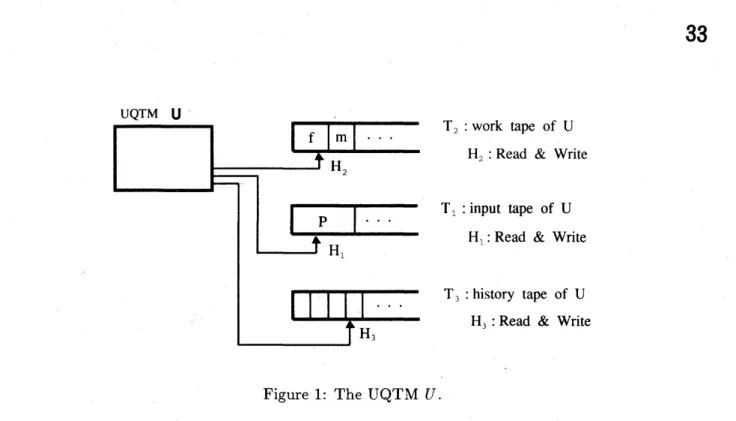
In this section, we show a method ofsolvingSAT in$O(n^{2})$ timeusing Deutsch’s UQTM under the assumption A[7]. In order to simulate a reversible universal DTM, the UQTM $U$ has an
input tape $T_{1}$, awork tape $T_{2}$, and a history tape $T_{3}$
.
Let $H_{1},$$H_{2}$, and $H_{3}$ be the heads onthe tapes $T_{1},$$T_{2}$, and $T_{3}$, respectively (see Figure 1).As shown in Figure 1, the UQTM $U$ starts the execution given a logical formula $f$ and
the number $m$ of variables in $f$ on the work tape $T_{2}$, and the program $P$ to simulate on the input tape $T_{1}$
.
On the right-hand side of$P$, infinitely many blank symbols are written. Noticethat the length of the description of $P$ is a constant which is independent of the length of
an input given on $T_{2}$
.
The program $P$ consists of state transition rules of one-tape standardDTMs andsentences corresponding to the eight unitary transformations above. Let $V(n, i)$ be
the sentence corresponding to these unitary transformations, where $0\leq n\leq 7$. This sentence
represents that “apply the transformation $V_{n}$ on the ithbit of the work tape”.
In all configurations in a superposition, $U$ can simulate a single step of $M$ in the same
$T_{2}$ : work tape of $U$
$H_{2}$ :Read &Write
$T_{1}$ : input tape of $U$
$H_{1}$:Read
&Write
$T_{3}$ :history tape of $U$
$H_{3}$ :Read &Write
Figure 1: The UQTM $U$.
until it finally halts, and is represented as a function of the length of the input (in this case,
the tdtal length of the descriptions of$f$ and $m$) given on $T_{2}$
.
Theorem 3.1 Under the assumption $A$, the UQTM $U$ can solve SAT in $O(n^{2})$ time, where
$n$ is the total length of the description of a logical formula $f$ whose satisfiability should be
decided and the description of the number of variables in $f$
.
sketch of proof In the sequel, we construct a program $P$ that $U$ simulates in order to
solve SAT in $O(n^{2})$ time. Let us consider the satisfiability for an m-variable logical formula
$f(x_{1}, x_{2}, \ldots, x_{m})$, where $x_{i},$ $i=1,2,$ $\ldots,m$ are boolean variables.
The machine $U$ writes an assignments to the variables in the logical formula $f$ together
with the corresponding valueof$f$
on
the tape $T_{2}$. We show the program that $U$ will simulatein Figure 2. $\ln$ thesequel, we explain the behavior of $U$ according to this program.
1. The initial configuration
The descriptions of the logical formula $f$ and the number $m$ of the variables are given as input on the work tape$T_{2}$, and theprogram$P$that $U$simulatesis given on the input tape
$T_{1}$
.
In the sequel,weidentify a configuration of$U$ with a description ofan assignment tothe variablesin$f$and the corresponding value of$f$, which are writtenon the tape$T_{2}$ (this
description is written on the right-hand side of $f$ and $m$ on $T_{2}$). Let $[x_{1}],$
$\ldots,$$[x_{m}]$, and
$[x_{m+1}]$ be thebits correspondingto$x_{1},$ $\ldots,$$x_{m}$ and the value of$f$ under theassignment in
this configuration, respectively. In the sequel, we are indicating only $[x_{1}, \ldots, x_{m}, x_{m+1}]$ in $[T_{2}]$ as a configuration of $U$
.
Let$[0,0, \ldots, 0;0]\sim$
$m$
be the initial configuration of$U$
.
In order to simplify the presentation, we separate thebegin %%% Preparations of inputs 1 for $i=1$ to $m$ do 2 $V(4,i)$ od ; %%% Computation of$f$ 3 $x_{m+1}$ $:=f(x_{1}, \ldots, x_{m})$ ;
%%% Preparations for an observation 4 for $j=m$ to 1 do
5 $V(0,j)$
od
end.
Figure 2: The program that the UQTM $U$ simulates.
2. Preparations of inputs
There exist $2^{m}$ different assignments for $m$ variables of$f$
.
Initially, $U$ makes asuperpo-sition ofconfigurationscorresponding to all of these assignments. $U$ will perform this by
applying
$V_{4}= \frac{1}{\sqrt{2}}(\begin{array}{l}1-111\end{array})$
to each bit corresponding to $m$ variables in order. $U$ can execute the transformation
by $V_{4}$ in a single step. In the execution ofthe first for loop, the initial configuration is
transformed as follows:
$[0,0, \ldots, 0;0]^{\bigcup_{x_{1_{arrow}^{\cup}}x_{m}}}\frac{1}{\sqrt{2^{m}}}\sum_{x_{1}=0}^{1}\sum_{x_{2}=0xm}^{1}\cdots\sum_{=0}^{1}[x_{1}, x_{2}, \ldots, x_{m}; 0]$.
Because $U$ can execute each transformation $\bigcup_{x}$
: in a single step, it can execute all the
transformations $\bigcup_{x_{1}}$, $\bigcup_{x_{m}}$ in $m$ steps.
3. Computation of$f$
Let $U_{f}$ be a transformation corresponding to the computation of the value of the logical
formula $f$, then
$\frac{1}{\sqrt{2^{m}}}\sum_{x_{1}=0}^{1}\sum_{x_{2}=0x}^{1}\cdots\sum_{m^{=0}}^{1}[x_{1}, x_{2}, \ldots, x_{m}; 0]$
$arrow\frac{1}{\sqrt{2^{m}}}\sum_{x_{1}=0}^{1}\sum_{x_{2}=0xm}^{1}\cdots\sum_{=0}^{1}[x_{1}, x_{2}, \ldots, x_{m}; f(x_{1}, x_{2}, \ldots, x_{m})]\equiv\psi U_{f}$.
In order to execute the third line of the program, $U$ simulates aprogram of a one-tape
standardDTM $M_{f}$ computing the values of$f$
.
$U$ simulates $M_{f}$, regarding$T_{2}$ as the tape4. Preparations for an observation
The machine $U$ executes the reverse transformation of the one executed in the
prepara-tions of inputs by applying
$V_{0}= \frac{1}{\mathscr{J}_{2}}(\begin{array}{ll}1 1-1 1\end{array})$
to the bits corresponding to the $m$ variables, from $[x_{m}]$ to $[x_{1}]$ in order. Because $U$
can execute a transformation by $V_{0}$ in a single step, it can execute the for loop of the
fourth line in Figure 2 in $m$ steps. In this transformation the superposition $\psi$ of $U’ s$
configurations will be transformed as follows:
(a) Ifthe values of$f$ for $2^{m}$ different assignments are all $O’ s,$ $\psi$ will be transformed to
one configuration $[0,0, \ldots, 0;0]$
.
(b) If the values of$f$ for $2^{m}$ different assignments are all l’s, $\psi$ will be transformed to
one configuration $[0,0, \ldots, 0;1]$
.
(c) Otherwise, $\psi$ will be transformed to a superposition of several configurations.
An Observation
When $U$ completes all the computaions above, we will observe whether there exists a
configu-ration$c_{0}=[0,0, \ldots, 0;1]$ intheflnallyobtained superpositionof$U’ s$configurations. If$c_{0}$ exists
in thesuperposition, we concludethat $f$is satisfiable, and if not,unsatisfiable. Thecorrectness
of this decision is shown by the claim below.
Claim $f$ is satisfiable if and only if there exists the configuration $[0,0, \ldots, 0;1]$ in
the finally obtained superposition of configurations.
The Time Complexity of UQTM $U$
Since the second line in Figure
2
is executed $m$ times in total, $U$ can execute the first forloop within$O(m)$ steps. As mentioned above, $U$ can execute the third line within $O(n^{2})$ time. Finally, $U$ can also execute the for loop of the fourth line within $O(m)$ steps. Therefore, $U$
can execute the procedure in Figure 2 within $O(n^{2})$ steps in total. $\square$
Definition [4] A language $L$ isinthe class EQP (exactor
error-free
quantum polynomial time$)$ if there exists a QTM with a distinguished acceptance tape cell, and a polynomial$p$, such
that given any string $x$ as input, observing the acceptance cell at time $p(n)$ correctly classifies $x$ with respect to$L$. More generally, alanguage $L$ is inthe class BQP (bounded-error quantum
polynomialtime) if this classificationcanbe accomplished with probability greater than 2/3[4]. Corollary 3.1 Under the assumption $A$, NP $\subseteq$ EQP.
Example In Figure 3, we show the change of the superpositions of configurations in the case
$\wedge^{[0,0;0]}$ $\wedge^{\frac{1}{\sqrt{2}}([0,0’ 0]}$ $+$ $\wedge^{[1,0;0\rfloor)}$ $\}o(n)$ time $\frac{1}{\mathcal{F}_{2}^{2}}([0,0;0]+[0,1;0]+[1,0;0]+[1,1;0])$
$u$
ComPutation
of $f$ $\}o(n^{2})$ time$\frac{1}{\sqrt{2}2}([0,0;1]+\lceil 0,1;0]+[1,0;0]+[1,1;1])$
$\frac{1}{1\overline{2^{3}}}$ (
$[0,0;1]\dashv 0,1;1]+[0,0;0J+[0.1;0]!$
[1,0;0]-[1,1;0]+[1,o;月 $+[1,1;1]$) $\}o(n)$ time
$\frac{1}{\sqrt{2}2}(\underline{[0,0;1]}+[0,0;0]![1,1;0]+[1,1;1])$
Figure 3: The change of the superposition of configurations of the UQTM $U$.
Acknowledgements The authors would like to express their sincere thanks to Professor
Kojiro Kobayashi at the Tokyo Institute ofTechnology forhis detailedcomments ona previous
version of this paper.
References
[1] Y. Aharonov, J. Anandan and L. Vaidman, “Meaning of the Wave Function”, Phys. Rev.,
A 47, pp. 4616-4626, 1993.
[2] C. H. Bennett, “Logical Reversibility of Computation”,$IBM$J. Res. Dev., 17, pp. 525-532,
1973.
[3] P. A. Benioff, “Quantum Mechanical Hamiltonian Models of Discrete Processes That Erase Their Own Histories
:
Application to Turing Machines, Int. J. Theor. Phys., 21, pp.177-201, 1982.
[4] E. Bernstein and U. Vazirani, “Quantum Complexity Theory”, Pro$c$
.
of 25th $ACM$ Sym-posium on Theo$ry$ of$Com$puting, pp. 11-20, 1993.[5] D. Deutsch, “Quantum Theory,the Church-Turing Principle and the Universal Quantum Computer”, Proc. R. Soc. Lond., A 400, pp. 97-117, 1985.
[6] D. Deutsch and R. Jozsa “Rapid Solution of Problems by Quantum Computation”, Proc.
$R$
.
Soc. $Lond.$, A 439, pp. 553-558, 1992.[7] 三原孝志, 西野哲朗, “量子コンピュータを用いた NP 完全問題の多項式時間解法