JAIST Repository: A Collaborative Filtering based Approach for Recommender Systems [課題研究報告書]

全文

(1)JAIST Repository https://dspace.jaist.ac.jp/. Title. A Collaborative Filtering based Approach for Recommender Systems [課題研究報告書]. Author(s). 康, 高熙. Citation Issue Date. 2020-03. Type. Thesis or Dissertation. Text version. author. URL. http://hdl.handle.net/10119/16432. Rights Description. Supervisor:Huynh Nam Van, 先端科学技術研究科, 修士（情報科学）. Japan Advanced Institute of Science and Technology.

(2) Master’s Research Project Report. A Collaborative Filtering based Approach for Recommender Systems. KANG Gaoxi. Supervisor. Huynh Nam Van. Graduate School of Advanced Science and Technology Japan Advanced Institute of Science and Technology (Information Science). 02-2020.

(3) Abstract In recent decades, with the continuous development of technology based on information systems and big data, more and more fields have been started the research and applications of personalized recommendation technologies. With the rapid growth of Internet business data, the processing capacity’s demand is also in an increasing trend. Accompanied by the fast growth of customer information is that how to use it effectively has become one of the issues that need to be paid attention to. In this report, we first introduce an overview of recommender systems consisting of its definition, theoretical basis, typical approaches, and implementation. Besides, we present solid background knowledge that is used in these systems such as similarity functions and k-Nearest Neighbor, Gradient Descent and Artificial Neural Networks, some standard evaluation metrics for a recommender system. We then applied the previous research to implement three different typical algorithms based on collaborative filtering. They are item-based k-Nearest Neighbors (i-kNN), Alternating Least Square (ALS), and Neural Network-based collaborative filtering recommender systems (NeuNet). After that, we conduct experiments on a public dataset from Netflix called MovieLens, which contains user information, item information, and the interaction between users and items (e.g., ratings, comments, etc.). The comparison between these algorithms’ performance also is considered. Through the experimental results, we found that recommendations from the item-based k-Nearest Neighbors approach are less diverse than those from the approach of Alternating Least Square, which can bring “surprise” recommendations to the users. From the statistic point of view, the Root Mean Square Error (RMSE) of the Neural Network based Recommender System is a little better. This result gives us more reference in the practical applications, thus providing a direction on the modern approaches for recommender systems. Keywords: Recommender System; Collaborative Filtering; Neural Network; kNearest Neighbors; Alternative Least Square. i.

(4) Contents Chapter1 Introduction ............................................................................................................. 1 1.1 Recommender Systems: an overview ................................................................................. 1 1.2 Typical approaches in Recommender Systems .................................................................... 1 1.2.1 Content-based methods .............................................................................................. 2 1.2.2 Collaborative filtering methods ................................................................................... 4 1.2.2.1 Memory-based methods ....................................................................................... 5 1.2.2.2 Model-based methods .......................................................................................... 6 1.2.3 Hybrid recommender system ...................................................................................... 7 1.3 Report objectives & Structure ........................................................................................... 7 Chapter 2 Background ............................................................................................................ 9 2.1 Similarity functions .......................................................................................................... 9 2.1.1 Minkowski(Euclidian, Manhattan, Chebyshev) ............................................................ 9 2.1.2 Cosine Similarity & Pearson Correlation ................................................................... 10 2.2 k-Nearest Neighbors ........................................................................................................11 2.3 Gradient Descent ........................................................................................................... 12 2.4 Artificial Neural Network ............................................................................................. 15 2.4.1 The structure of a typical ANNs ................................................................................ 16 2.4.1.1 The artificial neuron .......................................................................................... 16 2.4.1.2 Nodes ............................................................................................................... 16 2.4.1.3 The bias ............................................................................................................ 18 2.4.1.4 Putting the structure together .............................................................................. 18 2.4.1.5 The notation...................................................................................................... 19 2.4.2 Forward propagation ................................................................................................ 20 2.4.3 Backward propagation ............................................................................................. 21 2.5 Evaluation of Recommender Systems Results .................................................................. 22 Chapter 3 Problem Formulation and Approaches .................................................................... 24 3.1 Problem Formulation:..................................................................................................... 24 3.2 Item-based k-Nearest Neighbor Recommender System (i-kNN-RS) ................................... 25 3.2.1 Idea of i-kNN-RS:.................................................................................................... 26 3.2.2 Implementation Concerns ......................................................................................... 27 ii.

(5) 3.3 Alternating Least Square based Collaborative Filtering Recommender Systems(ALS-CFRS)29 3.3.1 Least Square Problem .............................................................................................. 30 3.4 Neural Network-based Recommender Systems ................................................................ 33 Chapter 4 Implementation and Experiments ........................................................................... 36 4.1 Data Description ............................................................................................................ 36 4.2 Data Exploration and Preprocessing ................................................................................ 37 4.3 Experimental Results...................................................................................................... 40 4.3.1 i-kNN-RS ................................................................................................................ 40 4.3.2 ALS-CFRS .............................................................................................................. 41 4.4 Neural Network-Based Collaborative Filtering Recommender Systems .............................. 43 Chapter 5 Conclusion & Future work ..................................................................................... 45 5.1 Conclusion .................................................................................................................... 45 5.2 Future works.................................................................................................................. 46 Bibliography ........................................................................................................................... 47. iii.

(6) List of Figures Figure 1.1: Typical paradigms for a recommender system………………...……...…2 Figure 2.1: Demonstration of k-Nearest Neighbors………………………………...12 Figure 2.2: Contour plot of a 3D surface…………………………………...…….…13 Figure 2.3: Gradient Descent with two parameters………………………...……….14 Figure 2.4: The convergence of Gradient Descent………………………...………..15 Figure 2.5: Sigmoid function…………………………………………..……….......16 Figure 2.6: Node with input……………………………………………..……….....17 Figure 2.7: Effect of adjusting weights……………………………………..………17 Figure 2.8: Effect of adjusting bias ………………………………………..……….18 Figure 2.9: Three layers of Neural Network……………………………….……….19 Figure 3.1: User-Item rating matrix…………………………………………….…..24 Figure 3.2: Demonstration of k-Nearest Neighbors………………………………...26 Figure 3.3: Code of turning data frame…………………………………………….28 Figure 3.4: Flowchart of item-based k-NN Recommender System……………..….28 Figure 3.5: Sparsity of a general dataset…………………………………………....30 Figure 3.6: Neural Network model in Keras………………………………………..34 Figure 3.7: Neural Network architecture………………………………………...…34 Figure 4.1: Example of the dataset…………………………………………………37 Figure 4.2: Count of the rating by users……………………………………….……37 Figure 4.3: Example of a specific movie…………………………………….……..38 Figure 4.4: Rating frequency plot…………………………………………….…….38 Figure 4.5: Recommendations of i-kNN-RS…………………………………….…41 Figure 4.6: Learning Curve of RMSE……………………………………………...42 Figure 4.7: Learning Curve of RMSE on different data partition…………………...44. iv.

(7) List of Tables Table 1.1: Contrast of memory-based methods…………………………………...…6 Table 2.1: Different distance function and example………………………………..10 Table 2.2: Algorithm of k-Nearest Neighbors search…………………………….....12 Table 3.1: Summarizes the notation used in this chapter……………………………25 Table 3.2: Algorithm of Item-based k-Nearest Neighbor Recommender System…..27 Table 3.3: Algorithm of Alternative Least Square Collaborative Filtering…………32 Table 3.4: Notations of network architecture……………………………………….33 Table 3.5: Contrast of different approach recommender system……………………35 Table 4.1: Information of the experiment dataset…………………………………..36 Table 4.2: Rating counts of movies…………………………………………………39 Table 4.3: Number of times for movies…………………………………………….39 Table 4.4: The value of hyper-parameters for i-kNN-RS…………………………...40 Table 4.5: The value of hyper-parameters for ALS-CF…………………………….41 Table 4.6: Grid search of rank and regularized parameter…………………………42 Table 4.7: Results of i-kNN-RS and ALS-CFRS…………………………………...43 Table 4.8: RMSE on ALS-CFRS and Neural Network-based CFRS……………….44. v.

(8) Chapter1 Introduction 1.1 Recommender Systems: an overview In today’s digital era, with the rise of many E-commerce platforms like Youtube, Amazon, Netflix, and many other web services, recommender systems have become more and more important in our lives. Definition: "A recommender system, or a recommendation system, is a subclass of information filtering system that seeks to predict the "rating" or "preference" a user would give to an item [wikipedia]. " Today's recommender systems are inevitable in our daily online journey and consumers are facing various choices of products at any time, from e-commerce with suggestions to articles of potentially interested buyers to online advertising which suggests users the right content to match their preferences. Technically, the recommender system is an algorithm that aims to recommend relevant items to users. The items may be movies, texts, products or others depending on business contexts. In this chapter, we will present an overview of the recommender system and their different examples. For each instance, we will introduce how they work, describe their theoretical basis, and discuss their advantages and disadvantages.. 1.2 Typical approaches in Recommender Systems In the first part, we introduce two typical paradigms of a recommender system: contentbased approach and collaborative filtering one and how they work. The next part will then describe various methods of collaborative filterings, such as user-based, item-based and matrix factorization. The overall of different paradigms for the recommender system is depicted in Figure 1.1.. 1.

(9) Recommender Systems. Content-based methods. Define a model for user-item interactions where users or items representations are given.. Memory based. Define no model for user-item interactions and rely on similarities between users or items in terms of observed interactions.. Model based. Define a model for user-item interactions where users and items representations have to be learned from interactions matrix. Collaborative filtering methods. Mix content based and collaborative filtering approaches. Hybrid methods. Figure 1.1: Typical paradigms for a recommender system [1]. 1.2.1 Content-based methods Content-based methods use additional information about users or items in making recommendations [2]. If we take the movie recommendation system as an example, this additional information can be, for example, age, gender, any other personal details of the user(like click on a specific item, purchasing item, etc.) as well as category, main actor, duration or other characteristics of the item. Then, the critical idea of a content-based method is to try to build a model based on available "features" that precisely explain observed user-item interactions. Retake users and movies as an instance; a good recommender system should reflect the fact that young women score higher on some movies, while young men score higher on others, and so on. If we try to get such a model, it's easy to make new predictions for users: we can utilize the user's profile (eg., age, gender, etc.). Basing on this information to determine the relevant movies, then make a recommendation list. In the content-based approach, the recommendation problem is transformed into a classification problem (predicting whether the user "likes" the product) or a regression problem (predicting the user's evaluation of the product). In both cases, we will set up the 2.

(10) model based on the available user or item features. If the classification or regression is based on user features, then we say the method is item-centered: modeling, optimization and calculation can be conducted "by item". In this case, we will build and learn a model item by item according to the features of users to try to answer "what is the probability that each user likes this item?" for regression. The model associated with each item will naturally be trained based on the data related to the items, and because many users have interacted with the items, it usually leads to quite powerful models. However, considering that the interaction of the learning model comes from each user, even if these users have similar features, their features may be different. This means that even if this method is more robust, it can be considered less personalized (more biased) than the user-centric methods. If we use item functionality, the method will be user-centric: modeling, optimization, and calculation can be done "by the user." Then, our goal is to train a model according to the features of the items, which tries to answer the following questions: "what is the probability that the user likes each item?" for regression. Then, we can attach the model to each user trained in the data: therefore, the model obtained is more personalized than the item-centric model, because it only considers the interaction from the users. However, in most cases, users interact with relatively few items, so the model we get is far less robust than the item-centered model. From a practical view, we should emphasize that in most cases, it is much more difficult to ask new users some information (users don't want to answer too many questions) than new items. That is because the person who added the item is interested in filling in this information in order to recommend its product to the appropriate user. We can also note that according to the complexity of expression relationships, the models we build are more or less complex, ranging from basic models (logical/linear regression for classification/regression) to deep neural network [3]. Finally, it should be mentioned that content-based methods can be neither user-centered nor item-centered: both information of users and items can be used in our model, for example, by stacking two eigenvectors 3.

(11) and passing them through the neural network architecture [4].. 1.2.2 Collaborative filtering methods The collaborative filtering methods of the recommender system are based on past interaction recorded between users and items to generate new recommendations. These interactions are stored in the “user-item interaction matrix.” Then, the main idea governing the collaborative filtering methods is that these past user-item interactions are sufficient to detect similar users or similar items, and predict based on the proximity of these estimates. The categories of collaborative filtering algorithms are divided into two subcategories, usually called memory-based methods and model-based methods. The memory-based approach works directly with the recorded interaction values and is basically on the nearest neighbor search. The model-based approach assumes a basic "build" model that interprets user-item interactions and attempts to discover such model in order to make new predictions. The main advantage of collaborative filtering algorithms is that they do not need information about users or items so that they can be used in many cases. Besides, the more users interact with the project, the more accurate the new suggestions are: for a set of fixed users and items, the new interaction recorded over time will bring new information and make the system more effective. However, since collaborative filtering only considers history interactions to make suggestions, it suffers some problem such as "Cold Start," "Scalability," "Sparsity": - Cold Start: when an item inserted into the catalog is minimal, even zero interactions. This causes some difficulty if recommender bases on those interactions to make recommendations - Scalability: when applying algorithms on a considerable dataset where the number of users and items are big enough. The current, practical datasets are almost extremely massive. 4.

(12) - Sparsity: in many practical E-commerce platforms such as Youtube, Netflix, Amazon, etc. The number of items & users is huge while the interaction between each (user, item) pairs is usually lacked. Because most users did not revise their purchasing products/items. This caused the problem of sparsity. It is unable to recommend anything to new users or items, and many users or items interactions are rarely effectively handled. This defect can be solved in different ways: such as random strategy [5] which is recommending random items to new users, maximum expectation strategy [6] which is recommending common items to new users or recommend new items to the most active users, exploratory strategy [7] which is recommending various items to new users or a group of new users and so on.. 1.2.2.1 Memory-based methods . User-based Collaborative Filtering To make new suggestions for users, the user-based method tries to identify users with. the most similar "interaction" to propose the most popular items among these users. This approach is called "user-centric" because it represents users and evaluates the distance between users based on their interaction with the items. Supposing we want to make recommendations for a given user. Firstly, each user can be represented by its interaction vector (row in the matrix) with different items. Then, we can calculate a certain "similarity" between interested users and all other users. This similarity measure makes two users who have similar interaction on the same item be regarded as intimate. Once we have calculated the similarity with each user pairs, we can keep k nearest neighbor to our users, and then suggest the most popular items. . Item-based Collaborative Filtering In order to make new suggestions to users, the idea of the item-based method is to find. items similar to those that users have already "actively" interacted with. If most users who interact with two items operate similarly, the two items are considered similar. This approach is called "item-centric" because it represents items based on the interaction 5.

(13) between users and them, and evaluates the distance between these items. Supposing we want to make recommendations for a particular user. Firstly, we consider his/her favorite products and represent them by an interaction vector (column in the matrix) with each user. Then, we can calculate the similarity between the "best item" and all other items. Once the similarity is calculated, we can keep k neighbors on the selected "best item", which is new for the users who are interested in, and recommend these items. Table 1.1 summarize the contrast between item-based and user-based in collaborative filtering [8]. Contrast. User-based Item-based. Search of similar. Users. Items. Variance. High. Low. Bias. Low. High. Table 1.1: Contrast of memory-based methods. 1.2.2.2 Model-based methods The model-based collaboration method only depends on the interaction information of users and items and assumes a potential model can explain these interactions. For example, the matrix decomposition algorithm decomposes the vast and sparse user-item interaction matrix into two smaller, dense matrices: user factor matrix (including user representation) multiplied by item factor matrix (including item representation). The main assumption behind matrix decomposition is that there is a relatively low dimensional feature space in which we can represent users and items, and we can get the interaction between users and items by the dot product of the corresponding dense vectors in that space. For example, we have a user-movie rating matrix. To simulate the interaction between users and movies, we can assume that: (1) Some features can describe movies well. (2) These features can also describe the user's preferences 6.

(14) However, we don't want to assign these capabilities to our model explicitly. On the contrary, we prefer to let the system discover these useful features and make its own representations to users and items. Since these features are not learned, the features extracted separately are of mathematical significance, but there is no intuitive explanation. However, it is not uncommon that this type of algorithm structure is very close to the intuitive decomposition that human can think of. In fact, the result of this factorization is that in terms of preferences, close to users and features close to items eventually have a close representation in the potential space.. 1.2.3 Hybrid recommender system Recent studies have shown that the hybrid approach of collaborative filtering and content-based filtering may be more effective in some cases [9]. There are several ways to implement hybrid methods, which are content-based prediction and collaborationbased prediction respectively [10], and then combine them to add content-based functions to collaboration based methods (and vice versa) or unify these methods into a method model [11]. Several studies compare the performance of the hybrid method with a pure collaboration-method and content-based approach and show that the hybrid method can provide more accurate suggestions than pure way [12]. These methods can also overcome some common problems in the recommender system, such as cold start and sparsity.. 1.3 Report objectives & Structure In this report, we will first study the typical approaches for a recommender system, then we reimplement these approaches and compare their performance in a specific context. To achieve this objective, we carry out subtasks as below: -. Survey about the general pattern of a recommender system: its definition, theoretical basis, approaches and implementation. This task is represented in Chapter 1.. -. Accomplish the background knowledge that needed to constitute a typical recommender system. These backgrounds include Gradient Descent & Artificial Neural Network, similarity measure & k-Nearest Neighbor, and valuation metrics for 7.

(15) the recommender system. They are presented in Chapter 2. -. Summarize three typical algorithm principles that provide the theoretical foundation for the whole report from different perspectives that will be present in Chapter 3.. -. Implementing the programs, conducting experiments on particular dataset, observing the result and make conclusions will be in Chapter 4 and Chapter 5.. 8.

(16) Chapter 2 Background This chapter will present a background knowledge of recommender systems. We will introduce the similarity functions and k-Nearest Neighbor, what is Gradient Descent and Artificial Neural Network in detail, and the evaluation method of the recommender system.. 2.1 Similarity functions Distance is a numerical measure of how far apart an object or point is. In physics or everyday use, distance can refer to physical length or an estimation basing on some predefined criteria. In mathematics, distance function or measure is a generalization version of physical distance’s concepts. Measurement is a function that runs according to a specific set of rules and is a way to describe the meaning of "close" or "far" between elements of a space.. 2.1.1 Minkowski(Euclidian, Manhattan, Chebyshev) Minkowski distance is a measure in norm vector space, which can be regarded as the generalization of Euclid distance, Manhattan distance and Chebyshev Distance. Minkowski distance of order p between two points 𝑋 = (𝑥1 , 𝑥2 , … … 𝑥𝑛 ) ∈ ℝ𝑛 and 𝑌 = (𝑦1 , 𝑦2 , … … 𝑦𝑛 ) ∈ ℝ𝑛 is defined as: 𝑝. 𝑑(𝑥, 𝑦) = √∑𝑛𝑖=1|𝑥𝑖 − 𝑦𝑖 |𝑝 When p equals different value, the formula can be defined as different distance functions, shown in table 2.1, if we take an example that = [0,6,0] 𝑦 = [2,8,9], the different distances are also shown in the table.. 9. (2-1).

(17) Manhattan Distance: 𝒑 = 𝟏 (L1-norm). Euclidian Distance: 𝒑 = 𝟐 (L2-norm). Chebyshev Distance: 𝒑 → +∞ (𝑳∝ -norm) 1 𝑝. 𝑛 𝒏. 2. 𝒅(𝒙, 𝒚) = ∑|𝒙𝒊 − 𝒚𝒊 |. 𝑑(𝑥, 𝑦) = lim (∑|𝑥𝑖 − 𝑦𝑖 |𝑝 ). 𝑛. 𝑝→+∞. 𝑑(𝑥, 𝑦) = √∑|𝑥𝑖 − 𝑦𝑖 |2. 𝒊=𝟏. 𝑖=1. 𝑖=1. = max{|xi − yi |} ∀i. 𝒅(𝒙, 𝒚) = |𝟎 − 𝟐| +. 𝑑(𝑥, 𝑦) =. |𝟔 − 𝟖| + |𝟎 − 𝟗| =13. 2. 𝑑(𝑥, 𝑦) = max{|0 − 2| +. √|0 − 2|2 + |6 − 8|2 + |0 − 9|2 |6 − 8| + |0 − 9|} = 9 =89. Table 2.1: Different distance function and example. 2.1.2 Cosine Similarity & Pearson Correlation Cosine similarity is usually useful for text data. It considers the angle between two vectors 𝑢 = [𝑢1 , 𝑢2 , … , 𝑢𝑛 ] and 𝑣 = [𝑣1 , 𝑣2 , … , 𝑣𝑛 ] ∈ ℝ𝑛 : ∑𝑛 𝑖=1 𝑢𝑖 ∗𝑣𝑖. 𝑢∙𝑣. Cosine(𝑢, 𝑣) = ‖𝑢‖∗‖𝑣‖ =. (2-2). 𝑛 2 2 √∑𝑛 𝑖=1 𝑢𝑖 √∑𝑖=1 𝑣𝑖. The range of similarity is from - 1 to 1, where 0 is orthogonal or decorrelated, and the middle value is similar or not. Example: Two documents consist of 10 words as below: car. bug. gid. dir. gid. ant. fox. fir. cat. log. u. 0. 6. 0. 0. 2. 0. 0. 0. 8. 9. v. 1. 0. 0. 0. 1. 0. 0. 3. 0. 0. Thus 𝑢 ∙ 𝑣 = 0 ∗ 1 + 6 ∗ 0 + ⋯ + 2 ∗ 1 + ⋯ + 9 ∗ 0 = 2 ‖𝑢‖ = √02 + 62 + ⋯ + 22 + ⋯ + 82 + 92 = 13.60 ‖𝑣‖ = √12 + ⋯ + 12 + ⋯ + 32 + ⋯ = 3.32 𝐂𝐨𝐬𝐢𝐧𝐞(𝑢, 𝑣) =. 𝑢∙𝑣 2 = = 0.044 ‖𝑢‖ ∗ ‖𝑣‖ 13.60 ∗ 3.32. These two documents are quite difference Pearson Correlation is a measure of the linear relationship between the attributes 10.

(18) of the two objects 𝑥 = [𝑥1 , 𝑥2 , … , 𝑥𝑛 ] and y = [𝑦1 , 𝑦2 , … , 𝑦𝑛 ] ∈ ℝ𝑛 : 𝑆𝑥𝑦. 𝑟(𝑥, 𝑦) = 𝑆. 𝑥 ∗𝑆𝑦. (2-3). 1. where 𝑆𝑥𝑦 = 𝑐𝑜𝑣𝑎𝑟𝑖𝑎𝑛𝑐𝑒 (𝑥, 𝑦) = 𝑛−1 ∑𝑛𝑖=1(𝑥𝑖 − 𝑥̅ )(𝑦𝑖 − 𝑦̅) 1. 𝑆𝑥 = 𝑆𝑡𝑎𝑛𝑑𝑎𝑟𝑑 𝑑𝑒𝑣𝑖𝑎𝑡𝑖𝑜𝑛 (𝑥) = √𝑛−1 ∑𝑛𝑖=1(𝑥𝑖 − 𝑥̅ )2 1. 𝑆𝑦 = 𝑆𝑡𝑎𝑛𝑑𝑎𝑟𝑑 𝑑𝑒𝑣𝑖𝑎𝑡𝑖𝑜𝑛 (𝑦) = √𝑛−1 ∑𝑛𝑖=1(𝑦𝑖 − 𝑦̅)2 𝑛. 1 𝑥̅ = 𝑚𝑒𝑎𝑛 (𝑥) = ∑ 𝑥𝑖 𝑛 𝑖=1 𝑛. 1 𝑦̅ = 𝑚𝑒𝑎𝑛 (𝑦) = ∑ 𝑦𝑖 𝑛 𝑖=1. Notice that 𝑟(𝑥, 𝑦) ∈ [−1, +1] , where +1 indicates total positive linear correlation, 0 means no linear correlation, and −1 indicates total negative linear correlation Example: if hours of study: 𝑥 = [8,8,6,5,7,6] Test score:. 𝑦 = [81,80,75,65,91,80]. Then: 𝑟(𝑥, 𝑦) = 0.648 which is a certain correlation between study hours and test scores.. 2.2 k-Nearest Neighbors k-Nearest Neighbor is a method of estimating the distance between an unseen object and a set of observed data in the attribute vector space. It is instance-based or lazy learning in which the classification function is only approximated locally, and all calculations are delayed until the actual classification process. An object can be classified via a majority vote of its k neighbors. As shown in Figure 2.1, if 𝑘 = 1, the object is assigned to its nearest neighbor's class.. 11.

(19) Figure 2.1: Demonstration of k-Nearest Neighbors [13] Table 2.2 illustrates a typical pattern of k-Nearest Neighbors' search. Algorithm: k-Nearest Neighbors //Goal: search the nearest neighbors data point of a target object //input： - target object - A set of labeled objects - Similarity measure 𝑑(𝑥,𝑦) - The value of k (usually 𝑘 = 1,3,5,7 …) //Output: Top k data that are nearest to the target object. 1. for each object in the dataset calculate d(target object, current object), insert the distance into a sorted list. 2. Pick the first k entries from the sorted collection. 3. Return the results in step 2. Table 2.2: Algorithm of k-Nearest Neighbors search. 2.3 Gradient Descent1 Gradient Descent is one of the well-known optimization algorithms in machine learning, especially deep learning. It has a good mathematic background and usually be used in training models. Mathematically, gradient descent’s goal is to minimize a convex function to a local optimal by adjusting its parameters which are the gradients of the function 1. https://builtin.com/data-science/gradient-descent. 12.

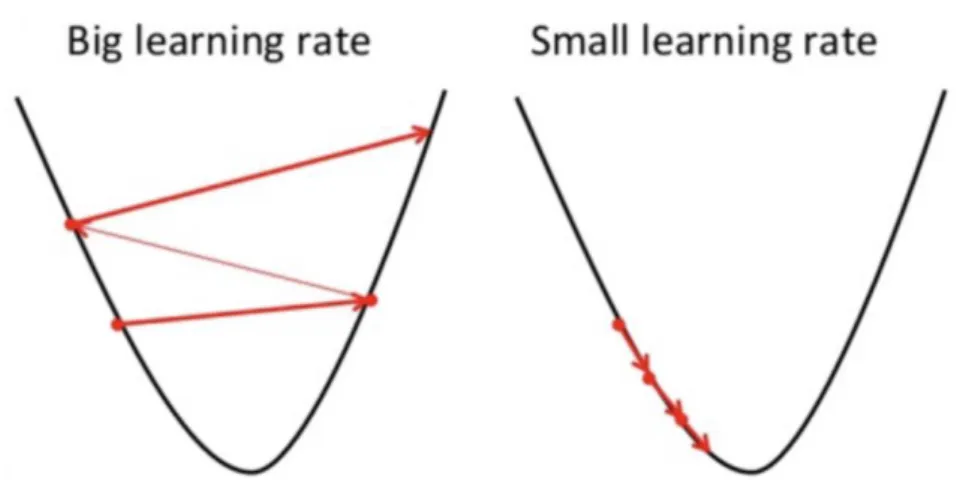
(20) This method is used to find the value of parameters, which minimize the cost function as much as possible. Gradient descent usually starts with an initial value of the parameters; then it iteratively adjusts the value from the gradient descent using the calculus to minimize the given cost function. For example that figure 2.2 shows a hill from top to bottom, and the red arrow is the climber's step. In this case, we can think of the gradient as a vector containing the direction to the hill’s peak that a climber should take to arrive at the highest point of the hill.. Figure 2.2: Contour plot of a 3D surface [wikipedia] The following equation describes the effect of gradient descent: 𝑏 is the climber's next position, and 𝑎 is his current location. A minus sign is the minimum part of the gradient drop. The middle 𝛾 is a waiting factor (e.g., known as learning rate) and the gradient (∆𝑓(𝑎)) is the direction of ascent. 𝑏 = 𝑎 − 𝛾∆𝑓(𝑎). (2-4). Therefore, the formula tells us the next position we need to climb, that is, the direction of the steepest ascent. We want to apply gradient descent to a Machining Learning problem, as shown in Figure 2.3. To minimize the cost function 𝐽 (𝑊, 𝑏) that means we 13.

(21) want to minimize the local cost function 𝐽 (𝑊, 𝑏) by adjusting 𝑊 & 𝑏. That figure 2.3 shows that the first two dimensions represent 𝑊 & 𝑏 respectively. The third one represents 𝐽 which is a convex function.. Figure 2.3: Gradient Descent with two parameters [wikipedia] Our goal is to find 𝑊 & 𝑏 values (marked with red arrows) corresponding to the local minimum value of the cost function. To arrive at the correct value, 𝑊 & 𝑏 usually are initialized at some random value. Then, the gradient descent will start at this position (near the bottom of the hill) and proceeds step by step in the steepest downward direction into a lower position. After a number of iterations, the cost function eventually ends up at hopefully the lowest point, called local minimal. To guarantee that the gradient decrease to a local minimum, learning rate should be set to an appropriate value not too high neither too low. This is vital because if the step size is too large, you may not be able to reach a local minimum, as it bounces back and forth between convex functions with gradient descent. On the other hand, if the learning rate is set to a too-small value, the function eventually reaches its local minimum but requiring a long time. Figure 2.4 illustrates these situations. 14.

(22) Figure 2.4: The convergence of Gradient Descent. 2.4 Artificial Neural Network2 Artificial Neural Networks(ANNs) are the computational models that try to imitate the human brain. They have shown huge advancements in a variety of Artificial Intelligence’s fields like Image Recognition, Voice Recognition, Robotics. The term "Neral" derives from the basic functional unit "neuron" of the human nervous system or nerve cells existing in the human brains and other parts of the human body. Artificial neural networks attempt to mimic and simplify these brain behaviors. A neural network is an algorithm that captures the hidden relationship between data points inside the dataset. Technically, it adapts itself to the input so that its resulting output is "best fit" the true ground label. 2 https://adventuresinmachinelearning.com/neural-networks-tutorial/#gradient-desc-opt. 15.

(23) 2.4.1 The structure of a typical ANNs 2.4.1.1 The artificial neuron Biological neurons are simulated in ANN by activation function. In the classification tasks, this activation function must have the "on" feature - in other words, once the input is higher than a specific value, the output should change state, i.e. from 0 to 1, or from −1 to 1, or from 0 to 0. This mimics the "opening" of biological neurons. A common activation function is usually the sigmoid function: 1. 𝑓(𝑧) = 1+exp(−𝑧). (2-5). Which looks like this:. Figure 2.5: Sigmoid function As can be seen from the above figure, this function is "activated," that is, when the input x is higher than a specific value, it moves from 0 to 1. Sigmoid colon function is not a stepping function, but the edge is "soft," and the output will not change immediately. This means that the function has a derivative, which is very important for the training algorithm.. 2.4.1.2 Nodes As mentioned before, biological neurons are connected to layered networks, and the 16.

(24) output of some neurons is the input of other neurons. We can express these networks as the connection layer of nodes. Each node uses multiple weighted inputs, and the activation function is applied to the sum of these inputs to generate the output. Consider the following figure:. Figure 2.6: Node with input in a Neural Network [14] The circle in figure 2.6 represents the node. Each node is then fed into the next layer, multiplied by the corresponding weight, sum up, then apply activation function to get the output at that layer unit. That output is shown as ℎ𝑤,𝑏 (𝑥) in figure 2.6. Mathematically: 𝑤1 𝑥1 + 𝑤2 𝑥2 + 𝑤3 𝑥3 + 𝑏. (2-6). Where 𝑤𝑖 here is the weight (known as parameters), They are variables that are changeable during learning and effects on the node’s output along with the input. If the value changes, the active function will change.. Figure 2.7: Effect of adjusting weights Here, changing the weight will shift the output slope of the active sigmoid function. If we want to model the different strengths of the relationship between input variables and 17.

(25) output variables, it is beneficial.. 2.4.1.3 The bias b is the weight of the +1 offset element - including this bias increases the flexibility of the node. If we only want to change the output when 𝑥 is higher than 1, that's where the bias occurs.. Figure 2.8: Effect of adjusting bias We can see, by changing the bias "weight," we can change when the node is active. Introducing a bias term, we can ensure that the node simulates a generic if function (𝑥 > 𝑧 ) and then 1, 0 otherwise. Without the bias term, we cannot change z in that if statement, it will always be stuck at about 0 . This is useful if we try to simulate conditional relationships.. 2.4.1.4 Putting the structure together A typical network architecture consists of a large number of artificial neurons, which are arranged in a series of layers. In a typical Artificial Neural Network, it contains different layers. These structures can take many different forms, but the most common simple network structure is usually composed of an input layer, hidden layers, and an output layer. An example of this structure is as follows:. 18.

(26) Figure 2.9: A Neural Network with two layers [15] - Input layer (layer 1): It contains units (artificial neurons) that take input from the outside world, on which the network will learn parameters or perform other processing. - Output layer (layer 3): it consists of units corresponding to information about how to learn any task. Hidden layer (layer 2) - these units are located between the input and output layers. The hidden layer’s job is transforming the input into some way that the output cell can use. As we can see, each node in layer 1 is connected to all nodes in layer 2. Similarly, for nodes in layer 2, there is a connection to layer 3 of a single output node. Each of these connections will have associated weights.. 2.4.1.5 The notation In the following equations, each of these weights is identified with the following (𝑙). notation: 𝑤𝑖𝑗 . 𝑖 refers to the number of nodes connected in layer 𝑙 + 1. 𝑗 refers to the number of nodes connected in layer l. So, the connection between node 1 in layer 1 and node 2 in layer 2, the weight (1). notation would be 𝑤21 . (𝑙). The notation of the bias weight is 𝑏𝑖 . ‘i’ is the node number in the layer 𝑙 + 1, which is the same as used for the regular 19.

(27) weight notation. So, the weight on the connection of the bias in layer 1 and the second (1). node in layer 2 is given by 𝑏2 . (𝑙). Finally, the node output notation is ℎ𝑗 . ‘j’ denotes the node number in layer 1 of the network. As can be observed in the three(2). layer network above, the output of node 2 in layer 2 has the notation of ℎ2 .. 2.4.2 Forward propagation The forward propagation can be treated to calculating the output from the input in neural networks. Below it is presented in equation form, we take the example in Figure 2.5: (2). (1). (1). (1). (1). (2). (1). (1). (1). (1). (2). (1). (1). (1). (1). ℎ1 = 𝑓(𝑤11 𝑥1 + 𝑤12 𝑥2 + 𝑤13 𝑥3 + 𝑏1 ). (2-7). ℎ2 = 𝑓(𝑤21 𝑥1 + 𝑤22 𝑥2 + 𝑤23 𝑥3 + 𝑏2 ). (2-8). ℎ3 = 𝑓(𝑤31 𝑥1 + 𝑤32 𝑥2 + 𝑤33 𝑥3 + 𝑏3 ) ℎ𝑊,𝑏 (𝑥) =. (3) ℎ1. =. (2) (2) 𝑓(𝑤11 ℎ1. +. (2) (2) 𝑤12 ℎ2. +. (2) (2) 𝑤13 ℎ3. (2-9) +. (2) 𝑏1 ). (2-10). In the equation above 𝑓(∗) refers to the node activation function, in this case, the (2). sigmoid function. The first line, ℎ1 (1). (1). is the first node’s output in the second layer, and. (1). (1). its inputs are 𝑤11 𝑥1 , 𝑤12 𝑥2 , 𝑤13 𝑥3 and 𝑏1 .These These inputs can be found in the three-layer connection diagram above. Sum them and then calculate the output of the first node by active function. Again, for the other two nodes in the second layer. The last line is the output of the only node in the third and final layer, which is the final output of the neural network. It can be seen that the final node does not adopt the weighted input variables ( 𝑥1 , 𝑥2 , 𝑥3 ), but adds the weighted bias to the second layer nodes (2). (2). (2). (ℎ1 , ℎ2 , ℎ3 ). Therefore, we can see the hierarchical nature of the artificial neural network in the equation. For calculation, there is a method that can write equations more compactly and calculate the forward process more effectively in the neural network. First, we can (𝑙). introduce a new variable 𝑧𝑖 , which is the total input of node i of layer 1, including the bias term. Therefore, for the first node in layer 2, z is equal to: 20.

(28) (2). (1). (1). (1). (1). (1). (1). 𝑧1 = 𝑤11 𝑥1 + 𝑤12 𝑥2 + 𝑤13 𝑥3 + 𝑏1 = ∑𝑛𝑗=1 𝑤𝑖𝑗 𝑥𝑖 + 𝑏𝑖. (2-11). where n is the nodes number of in layer 1. By this representation, the clumsy previous equations of the example three-layer network can be simplified as follows: 𝑧 (2) = 𝑊 (1) 𝑥 + 𝑏 (1). (2-12). ℎ(2) = 𝑓(𝑧 (2) ). (2-13). 𝑧 (3) = 𝑊 (2) ℎ(2) + 𝑏 (2). (2-14). ℎ𝑊,𝑏 (𝑥) = ℎ(3) = 𝑓(𝑧 (3) ). (2-15). Note that capital W is used to represent the matrix form of the weight. It should be noted that all elements of the above equation are now matrices or vectors. We can spread the calculation results to any number of layers in the neural network by the following summary: 𝑧 (𝑙+1) = 𝑊 (𝑙) ℎ(𝑙) + 𝑏 (𝑙). (2-16). ℎ(𝑙+1) = 𝑓(𝑧 (𝑙+1) ). (2-17). We can observe that the general forward propagation process, where the output of layer l becomes the input to its next layer 𝑙 + 1. We know that ℎ(1) is simply the input layer x and ℎ(𝑛𝑙) (where 𝑛𝑙 is the layers’ number in the network) is the output of the output layer. Note that in the above equation, we have removed the reference to the node number, and we can use matrix multiplication to do this more simply.. 2.4.3 Backward propagation The process of backward propagation is to learn the parameters of the network, which means to find the minimized settings (𝑊 (1) , 𝑏 (1) , 𝑊 (2) , 𝑏 (2) ) errors in our training data. We call the function of measurement error the cost function. The equivalent cost function of a training pair (𝑥 𝑧 , 𝑦 𝑧 ) in the neural network is as follows: 1. 1. 𝐽(𝑤, 𝑏, 𝑥, 𝑦) = 2 ‖𝑦 𝑧 − ℎ𝑛𝑙 (𝑥 𝑧 )‖2 = 2 ‖𝑦 𝑧 − 𝑦𝑝𝑟𝑒𝑑 (𝑥 𝑧 )‖. 2. (2-18). This shows the cost function of the 𝑧𝑡ℎ training sample, ℎ𝑛𝑙 is the last layer’s output of the neural network, which is the neural network output. ℎ𝑛𝑙 is represented as 𝑦𝑝𝑟𝑒𝑑 21.

(29) to highlight the prediction for a given 𝑥 𝑧 . The first. 1 2. is just a constant. When we. distinguish cost functions, we will sort things out, which will be done during backward propagation. Note that the formula for the above cost function applies to a single (x, y) training pair. We want to minimize the cost function among all m training pairs. So, we hope to find the minimum Mean Square Error (MSE) of all training samples: 1. 1. 1. 𝑚 𝑧 𝑛𝑙 𝑧 2 (𝑧) (𝑧) 𝐽(𝑤, 𝑏) = 𝑚 ∑𝑚 ,𝑦 ) 𝑧=0 2 ‖𝑦 − ℎ (𝑥 )‖ = 𝑚 ∑𝑧=0 𝐽(𝑤, 𝑏, 𝑥. (2-19). We train the weight of the network by using the cost function J and gradient descent. (𝑙). (𝑙). The gradient of each weight 𝑤𝑖𝑗 and bias 𝑏𝑖 (𝑙). (𝑙). 𝑤𝑖𝑗 = 𝑤𝑖𝑗 − 𝛼 (𝑙). (𝑙). 𝑏𝑖 = 𝑏𝑖 − 𝛼. 𝜕 (𝑙). 𝜕𝑤𝑖𝑗 𝜕. (𝑙). 𝜕𝑏𝑖. in the neural network is as follows:. 𝐽(𝑤, 𝑏). (2-20). 𝐽(𝑤, 𝑏). (2-21). Where 𝑤𝑛𝑒𝑤 = 𝑤𝑜𝑙𝑑 − 𝛼 ∗ ∇𝑒𝑟𝑟𝑜𝑟 . The left-hand side of this equation is the updated value of the weight, while the right-hand side is the old value of the weight. Again, we have an iterative process in which the weights are updated at each step basing on J (W, b).. 2.5 Evaluation of Recommender Systems Results The recommender system is a prediction model with algorithms. Usually, these algorithms are seeking to minimize the function error. Therefore, it is essential to measure the prediction error that they compare the expected results with the prediction results given by the model. To measure the accuracy of recommender system results, some of the most common prediction error measures are usually used, including Mean Absolute Error (MAE) and its related measures: Mean Square Error (MSE), Root Mean Square Error (RMSE) and normalized mean absolute error.. 22.

(30) 𝑀𝐴𝐸 =. 𝑀𝑆𝐸 =. ∑𝑛 𝑖=1|𝑟̂ 𝑢𝑖 −𝑟𝑢𝑖 | 𝑛. 2 ∑𝑛 𝑖=1(𝑟̂ 𝑢𝑖 −𝑟𝑢𝑖 ). 𝑛. 2 ∑𝑛 𝑖=1(𝑟̂ 𝑢𝑖 −𝑟𝑢𝑖 ). 𝑅𝑀𝑆𝐸 = √. 𝑛. (2-22). (2-23). (2-24). Where 𝑟̂𝑢𝑖 − 𝑟𝑢𝑖 is the difference between the predicted and the real value, for each n occurrence MAE measures the average size of errors in a set of predictions, regardless of their direction. It is the average of the absolute difference between the predicted value and the actual observed value in the test sample, where the weight of all individual differences is equal. RMSE is a secondary scoring rule, which can also measure the average magnitude of error. It is the square root of the average value of the squared difference between the predicted value and the actual observed value. In addition to these three indicators, two critical concepts also need to be considered: Precision and Recall. 𝑝𝑟𝑒𝑐𝑖𝑠𝑖𝑜𝑛 = 𝑅𝑎𝑐𝑎𝑙𝑙 =. |𝑅𝑒𝑐𝑜𝑚𝑚𝑒𝑛𝑑𝑒𝑑∩𝑅𝑒𝑙𝑒𝑣𝑎𝑛𝑡| |𝑅𝑒𝑐𝑜𝑚𝑚𝑒𝑛𝑑𝑒𝑑| |𝑅𝑒𝑐𝑜𝑚𝑚𝑒𝑛𝑑𝑒𝑑∩𝑅𝑒𝑙𝑒𝑣𝑎𝑛𝑡| |𝑅𝑒𝑙𝑒𝑣𝑎𝑛𝑡|. (2-25) (2-26). Precision is the ability to provide the relevant elements with the least amount of advice. Recall can find all relevant elements and recommend them to users.. 23.

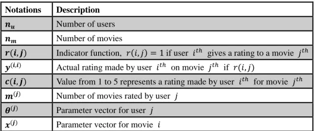
(31) Chapter 3 Problem Formulation and Approaches 3.1 Problem Formulation: Let’s take the problem of predicting movie ratings for the process of our formulation, although the general form is similar to this specific instance. Assume that there are 𝑛𝑢 users and 𝑛𝑚 movies. Each user gives a rating, which is a real number from 1 to 5, for all movies that he/she is interested in. Each movie receives a rating from all users. Formally, we get a matrix of size 𝑛𝑚 × 𝑛𝑢 where each row represents a list of ratings made by all users for a specific movie, and each column represents a list of ratings made by a particular user for all movies. As shown in Figure 3.1. Each cell in the matrix may receive unknown value which is denoted as a “?” because there are some users who did not rate for a movie. This is known as a sparse matrix.. Movie. Alice 5. Bob 5. Carol 0. Dave 1. Romance forever Cute puppies of love. 5 ?. ? 4. ? 0. 0 ?. Nonstop car chases Sword vs karate. 0 0. 0 0. 4 5. 4 ?. Love at last. … Figure 3.1: User-Item rating matrix. 24. ….

(32) Notations. Description. 𝒏𝒖. Number of users. 𝒏𝒎. Number of movies. 𝒓(𝒊, 𝒋). Indicator function, 𝑟(𝑖, 𝑗) = 1 if user 𝑖 𝑡ℎ gives a rating to a movie 𝑗 𝑡ℎ. 𝒚(𝒊,𝒊). Actual rating made by user 𝑖 𝑡ℎ on movie 𝑗 𝑡ℎ if 𝑟(𝑖, 𝑗). 𝒄(𝒊, 𝒋). Value from 1 to 5 represents a rating made by user 𝑖 𝑡ℎ for movie 𝑗 𝑡ℎ. 𝒎(𝒋). Number of movies rated by user 𝑗. 𝜽(𝒋). Parameter vector for user 𝑗. 𝒙(𝒋). Parameter vector for movie 𝑖 Table 3.1: Summarizes the notation used in this chapter. The goal is to efficiently infer these missing values so that the matrix “best reflects” the actual interaction between each movie and its corresponding users. 𝑇. Mathematically, for user 𝑖, movie 𝑗, predict: (𝜃 (𝑗) ) (𝑥 (𝑖) ). Equivalently, we want to learn: 𝜃 (𝑗) and 𝑥 (𝑖) for all 𝑖, 𝑗. In the following sections of this chapter, we will introduce some approaches for learning these missing values which are Item-based k-Nearest Neighbor Recommender System (ikNN-RS), Alternative Least Square based Collaborative Filtering (ALS-CF), and Neural Network-based Collaborative Filtering (Neural Network-CF).. 3.2 Item-based k-Nearest Neighbor Recommender System (i-kNN-RS) In this section, we introduce the item-based k-Nearest Neighbor Recommender System algorithm called i-kNN-RS. In chapter 4, we will show the experiment results of this model. i-kNN-RS is an easy-to-go model and usually plays the role of a very appropriate baseline for comparison between different recommender models. As shown in figure 3.2 and be introduced in chapter2, kNN is a non-parametric, lazy learning model. It uses a dataset consisting of the data points which are separated into groups to predict the value for a new instance. Also, note that kNN’s result much depends on the distance function. 25.

(33) In the case, that input training data are in a high dimensional space. kNN’s performance will commit the problem of the curse of dimensionality if kNN considers Euclidean distance as its objective function. Euclidean distance does not help in high dimensions, because all vectors are almost equidistant from the input query vectors (features of the target movie). Instead, the cosine similarity introduced in chapter 2 is entirely appropriate in this situation. Although the detail process of i-kNN-RS is depicted in Figure 3.2, we should introduce its key idea first.. Figure 3.2: Demonstration of k-Nearest Neighbors. 3.2.1 Idea of i-kNN-RS: The primary purpose of the item-based kNN-Recommender System is simple. It does not add any particular assumption on the data distribution; it much bases on the feature similarity between items. When making inference about the similarity between movies, kNN needs to compute the distance between the target movie and other movies in the dataset, then ranks the results in a descending order according to distance from each movie to the input target movie, and returns the top k nearest neighbor movies which are the most 𝑘 similar movies. The overall algorithm for i-kNN-RS is illustrated in Table 3.2.. 26.

(34) Algorithm: item-based k-NN Recommender System //Goal: Implement a recommender system bases on item-based k-NN search //Input: - 𝑘: number of nearest neighbors - 𝑖𝑛𝑝𝑢𝑡_𝑚𝑜𝑣𝑖𝑒: the target movie for recommending - a matrix of size 𝑚 × 𝑛 consisting of all ratings of 𝑚 movies by 𝑛 users - 𝑑𝑖𝑠𝑡𝑎𝑛𝑐𝑒_𝑡𝑦𝑝𝑒: distance function type, e.g., Euclidian, Manhattan, cosine, etc. //Output: Top 𝑘 movies that are nearest to the 𝑖𝑛𝑝𝑢𝑡_𝑚𝑜𝑣𝑖𝑒. 1. for every 𝑚𝑜𝑣𝑖𝑒𝑖 in the dataset do 2. calculate and store the distance 𝑑(𝑚𝑜𝑣𝑖𝑒𝑖 , 𝑖𝑛𝑝𝑢𝑡_𝑚𝑜𝑣𝑖𝑒) 3. Sort the movies in a descending order regarding its distances 4. Pick up and return the top 𝑘 movies at step #3 5. end item-based k-NN Recommender System Table 3.2: Algorithm of Item-based k-Nearest Neighbor Recommender System. 3.2.2 Implementation Concerns This section describes some critical concerns related to the implementation of i-kNNRS. First, the rating input data need to be transformed into an appropriate format that can be feed into the i-kNN-RS model. The data should be in a 2D array of size 𝑚 × 𝑛, where 𝑚, 𝑛 represent for the number of movies and the number of users, respectively. To reshape the data frame of ratings, we format movies as rows and users as columns. Then missing values need to be filled in with zeros because of applying linear algebra operations which are computing the distances between vectors. We can now consider this new data frame as a feature vector of each movie in the input dataset. One important observation here is that the matrix representing the movie extremely sparse. We should not feed the entire data with mostly floating zero numbers into the ikNN-RS model. To achieve the calculation efficiency and consuming less memory units,. 27.

(35) the data frame should be transformed into a SciPy sparse matrix3 and being implemented as shown in Figure 3.3.. Figure 3.3: Code of turning data frame. Figure 3.4: Flowchart of item-based k-NN Recommender System 3 SciPy sparse matrix is a python package providing tools for creating sparse matrices using multiple data structures, as well as tools for converting a dense matrix into a sparse one. 28.

(36) In chapter 4, we will conduct experiments on this model and consider its performance as a baseline with the other ones.. 3.3 Alternating Least Square based Collaborative Filtering Recommender Systems(ALS-CFRS) In the previous section, we formulated and introduced a baseline recommender system called i-kNN-RS, as well as provided some implementation concerns for it. Although ikNN-RS is easy to be implemented, it is evident that there are some limitations such as “cold-start problem” and “scalability issue.” The problem of item cold-start occurs when a movie inserted into the catalog is minimal, even zero interactions. This causes some difficulty if recommender bases on those interactions to make recommendations The issue of scalability occurs when applying i-kNN-RS on a considerable dataset where the number of users and items are big enough. The current, practical datasets are almost extremely massive, e.g., MovieLens_Datasets These two above problems are prevalent challenges for a typical collaborative filtering recommender system. They appear naturally along with the user-item (or item-user) interaction matrix where each cell 𝑐(𝑖, 𝑗) in the matrix represents a rating of the user 𝑖 and movie 𝑗. In practical applications, one item (e.g., movie) receives very few or even no ratings by all users. So that we are coping with an extremely sparse matrix with sparsity level is more than 99% as illustrated in Figure 3.5.. 29.

(37) Figure 3.5: Sparsity of a general dataset To deal with the problem, this section presents a little more sophisticated approach called ALS-CFRS which is based on a well-known mathematical technique called lowrank Matrix Factorization.. 3.3.1 Least Square Problem Before discussing in detail Alternative Least Square Collaborative Filtering let’s briefly revise the least-squares problem (in particular, a norm 𝐿2 -regularized least squares problem). Mainly, our goal in the least-squares problem by the language of linear algebra is to minimize the cost function of the form:. argmin(‖𝑦 − 𝑋𝑤‖22 + 𝜆‖𝑤‖22 ). (3-1). 𝑤. where 𝑋 is a feature matrix, 𝑋 ∈ ℝ𝑚×𝑑 ; 𝑦 is the target value, 𝑦 ∈ ℝ𝑚×1 ; 𝑤 is the parameter of the model 𝑤 ∈ ℝ𝑑×1 ; and 𝜆 is the adjusting rate for avoiding overfitting. In the language of linear algebra, the optimal solution of linear regression can be found analytically as follow: 30.

(38) 𝑤 = (𝑋 𝑇 𝑋 + 𝜆𝐼)−1 𝑋 𝑇 𝑦. (3-2). We can further expand this approach for multi-linear regression over multiple target 𝑌 = {𝑦1 , 𝑦2 , … , 𝑦𝑛 } using the same feature matrix. The solution parameter is similar but now is put all together within a matrix as below: 𝑊 = (𝑋 𝑇 𝑋 + 𝜆𝐼)−1 𝑋 𝑇 𝑌. (3-3). In practice, we rarely get to use this elegant analytical approach because it requires inverting a square matrix of size 𝑑 where 𝑑 usually takes a value from thousands to millions. And this is not a feasibly right approach because the inversion of a huge-size matrix is not only computationally expensive but numerically unstable. Fortunately, despite being rarely used in practical problems, this analytical approach is possible for recommender systems as we will show shortly as below. Recall from the problem definition section that for user 𝑖, movie 𝑗, we want to predict: 𝑇. (𝜃 (𝑗) ) (𝑥 (𝑖) ). Equivalently, we want to learn: 𝜃 (𝑗) and 𝑥 (𝑖) for all 𝑖, 𝑗. Note that the role of users and movies is exchangeable. That means if the movie parameter 𝑥 (𝑖) is given, then 𝜃 (𝑗) can be learned by minimizing the following leastsquare lost function for a particular user 𝜃 (𝑗) : 2. 𝑇. 1. 𝜆. (𝑗) 2. ∑𝑖:𝑟(𝑖,𝑗)=1 ((𝜃 (𝑗) ) (𝑥 (𝑖) ) − 𝑦 (𝑖,𝑗) ) + ∑𝑛𝑘=1 (𝜃𝑘 ) min (𝑗) 2 2. (3-4). 𝜃. To learn 𝜃 (1) , 𝜃 (2) , … , 𝜃 (𝑛𝑢) for all users, the total cost function turns out to be: min (2). 𝜃(1) ,𝜃. ,…,𝜃(𝑛𝑢. 2. 𝑇. 1. (𝑗) 2. 𝜆. 𝑢 𝑢 ∑𝑛𝑗=1 ∑𝑖:𝑟(𝑖,𝑗)=1 ((𝜃 (𝑗) ) (𝑥 (𝑖) ) − 𝑦 (𝑖,𝑗) ) + ∑𝑛𝑗=1 ∑𝑛𝑘=1 (𝜃𝑘 ) (3-5) )2 2. Similarly, if the user parameter 𝜃 (𝑗) is given, then 𝑥 (𝑖) can be learned by minimizing the following least square cost function for a particular movie 𝑥 (𝑖) : 1. 2. 𝑇. (𝑖) 2. 𝜆. ∑𝑗:𝑟(𝑖,𝑗)=1 ((𝜃 (𝑗) ) (𝑥 (𝑖) ) − 𝑦 (𝑖,𝑗) ) + ∑𝑛𝑘=1(𝑥𝑘 ) min (𝑖) 2 2. (3-6). 𝑥. To learn 𝑥 (1) , 𝑥 (2) , … , 𝑥 (𝑛𝑚) for all users, the total cost function turns out to be: 𝑥 (1) ,𝑥. min (2). ,…,𝑥 (𝑛𝑚. 1. 𝑇. 2. 𝜆. 2. 𝑚 𝑚 ∑𝑛𝑖=1 ∑𝑗:𝑟(𝑖,𝑗)=1 ((𝜃 (𝑗) ) (𝑥 (𝑖) ) − 𝑦 (𝑖,𝑗) ) + ∑𝑛𝑖=1 ∑𝑛𝑘=1(𝑥𝑘(𝑖) ) (3-7) )2 2. Combining (3-5) and (3-7), give us the objective cost function as below:. 31.

(39) 2. 𝑇. 1. 𝜆. (𝑖) 2. 𝑛. 𝑚 ∑𝑛𝑘=1(𝑥𝑘 ) + min 𝐽(Θ, 𝑋) = min 2 ∑(𝑖,𝑗):𝑟(𝑖,𝑗)=1 ((𝜃 (𝑗) ) (𝑥 (𝑖) ) − 𝑦 (𝑖,𝑗) ) + 2 ∑𝑖=1. Θ,𝑋. Θ,𝑋. (𝑗) 2. 𝜆. ∑𝑛𝑢 ∑𝑛 (𝜃𝑘 ) 2 𝑗=1 𝑘=1. (3-8). Now we can employ gradient descent to learn both 𝜃 (𝑗) and 𝑥 (𝑖) simultaneously with the update rule for every 𝑗 = 1,2, … , 𝑛𝑢 , 𝑖 = 1,2, … , 𝑛𝑚 as below: (𝑖). (𝑖). 𝑇. (𝑗). (𝑖). (𝑗). (𝑗). 𝑇. (𝑖). (𝑗). 𝑥𝑘 = 𝑥𝑘 − 𝛼 (∑𝑗:𝑟(𝑖,𝑗)=1 ((𝜃 (𝑗) ) (𝑥 (𝑖) ) − 𝑦 (𝑖,𝑗) ) 𝜃𝑘 + 𝜆𝑥𝑘 ) 𝜃𝑘 = 𝜃𝑘 − 𝛼 (∑𝑖:𝑟(𝑖,𝑗)=1 ((𝜃 (𝑗) ) (𝑥 (𝑖) ) − 𝑦 (𝑖,𝑗) ) 𝑥𝑘 + 𝜆𝜃𝑘 ). (3-9) (3-10). The overall algorithm is described in Table 3.3. Algorithm: Alternative Least Square Collaborative Filtering Recommender Systems //Goal: Implement a recommender system bases on ALS-CFRS //Input: - 𝑛: number of components for user parameters and movie parameters - a matrix of size 𝑛𝑚 × 𝑛𝑢 consisting of all ratings of 𝑛𝑚 movies by 𝑛𝑢 users //Output: predicting the rating of a user 𝜃 (𝑗) and a movie 𝑥 (𝑖) 1. Initialize 𝜃 (1) , 𝜃 (2) , … , 𝜃 (𝑛𝑢 ) & 𝑥 (1) , 𝑥 (2) , … , 𝑥 (𝑛𝑚) to small random values. 2. Minimize 𝐽(𝜃 (1) , 𝜃 (2) , … , 𝜃 (𝑛𝑢) , 𝑥 (1) , 𝑥 (2) , … , 𝑥 (𝑛𝑚) ) using gradient descent (𝑖). (𝑖). 𝑥𝑘 = 𝑥𝑘 − 𝛼 ( ∑. 𝑇. (𝑗). (𝑖). 𝑇. (𝑖). (𝑗). ((𝜃 (𝑗) ) (𝑥 (𝑖) ) − 𝑦 (𝑖,𝑗) ) 𝜃𝑘 + 𝜆𝑥𝑘 ). 𝑗:𝑟(𝑖,𝑗)=1. (𝑗). (𝑗). 𝜃𝑘 = 𝜃𝑘 − 𝛼 ( ∑. ((𝜃 (𝑗) ) (𝑥 (𝑖) ) − 𝑦 (𝑖,𝑗) ) 𝑥𝑘 + 𝜆𝜃𝑘 ). 𝑖:𝑟(𝑖,𝑗)=1. 3. For a user with parameter 𝜃 (𝑗) and a movie with parameter 𝑥 (𝑖) , predict a 𝑇. star rating of (𝜃 (𝑗) ) (𝑥 (𝑖) ). 4. End Table 3.3: Algorithm of Alternative Least Square Collaborative Filtering. Note that in the language of linear algebra, this problem is known as a low-rank matrix factorization problem. The detail of low-rank matrix factorization is beyond the scope of 32.

(40) this thesis. Chapter 4 will describe the experiment results of this approach. Furthermore, similar to other machine learning algorithms, ALS-CFRS has its own set of hyperparameters such as: rank: the number of hidden factors in our ALS-CFRS model (defaults: 10) regParam is the regularization parameter (defaults: 1.0) We may need to tune these hyper-parameters via hold-out validation or grid search to get the final ALS-CFRS model. In the tuning process of ALS-CFRS, we applied the grid search. Particularly, after tuning, we found the best choice for hyper-parameters are 𝑟𝑒𝑔𝑃𝑎𝑟𝑎𝑚 = 0.05 and 𝑟𝑎𝑛𝑘 = 20.. 3.4 Neural Network-based Recommender Systems One of the disadvantages of the ALS-RS is that it just considers the linear relationship between data points in the dataset. In this section, we consider a much more complex model which bases on Neural Network to copy with non-linear relationships within the dataset. Because the background of the Neural Network was introduced in chapter 2, here we present the architecture network that will be used in this report. Table 3.4 summarize all notations used for defining network architecture Notations. Description. num_users. number of users. num_items. number of movies. MF_dim. int, embedded dimension for user and item vector. MF_reg. tuple of float, 𝐿2 -regularization of MF embedded layer. MLP_layers. list of int, each element is hidden unit number for each MLP layer, except for the first element. First element is the sum of user latent vector and item latent vector. MLP_regs. list of int, each element is the 𝐿2 -regularization parameter for each layer in the neural network model Table 3.4: Notations of network architecture. We declare the neural network model via Keras4 library as below: 4 Keras is an open-source library written in Python, designed to enable fast 33.

(41) Figure 3.6: Neural Network model in Keras Figure 3.7 summarizes our neural network architecture. Figure 3.7: Neural Network architecture. experimentation with deep neural networks, it focuses on being user-friendly, modular, and extensible [wikipedia].. 34.

(42) Next, we train the model via Adam5 optimization algorithm with some parameters such as 𝐵𝐴𝑇𝐶𝐻_𝑆𝐼𝑍𝐸 = 64 𝐸𝑃𝑂𝐶𝐻𝐸𝑆 = 30 𝑉𝐴𝐿𝐼𝐷𝐴𝑇𝐼𝑂𝑁_𝑆𝑃𝐿𝐼𝑇 = 25% After training the model, we estimate its performance on the test set via the estimator Root Mean Square Error (RMSE). The experimental results will be discussed in chapter 4. Note that the process of selecting an appropriate network architecture is known as hyper-parameter tuning and usually not easy to cope with. We leave that problem as future work in this report. In conclusion, this chapter introduced three different approaches for a recommender system such as i-kNN-RS, ALS-RS, and Neural Network-based RS. Table 3.5 summarized the advantages and disadvantages of these approaches. Approach. i-kNN-RS. ALS-CFRS. Neural Network-RS. Advantages. Disadvantages Much depends on distant function and Simple, easy to be the value of 𝑘. implemented Simply filling zero to the missing No training phase values, so that does not reflect the genuine relationship inside the dataset Has a well mathematical Not work well for datasets consisting of definition so that there is an a non-linear relationship between data analytical solution points Efficient for problem with medium dataset Require more resources like training Able to consider complex times. relationships between data A large number of hyper-parameters points inside the dataset need to be tuned Table 3.5: Contrast of different approach recommender system. 5 Adam optimization algorithm is a kind of stochastic gradient descent optimizer provided by Keras library. 35.

(43) Chapter 4 Implementation and Experiments 4.1 Data Description The experiment in this chapter uses MovieLens6 dataset which consists of two main files, movies.csv, and ratings.csv. The dataset describes a list of ratings and free-text tagging activities made by users for movies. In total, there are 27,753,444 ratings and 1,108,997 tags across 53,098 unique movies. These data created by 283,228 individual users during the time (1995/01/09-2018/09/26). The dataset has eliminated demographic information. A hash id identifies each user without any other information. Table 4.1 summarizes the general information of this dataset. Data Description Number of movies. 53,098. Number of users. 283,228. Number of ratings. 27,753,444. Number of tags. 1,108,997. Time of collecting the dataset. 1995/01 – 2018/09. Table 4.1: Information of the experiment dataset. Figure 4.1 extracts and shows some instances from the dataset. 6 This is a public dataset available at https://grouplens.org/datasets/movielens/latest/ 36.

(44) Figure 4.1: Example of the dataset. 4.2 Data Exploration and Preprocessing Before executing the program, let’s explore some properties of the data. Firstly, we want to get the counts of each rating from the file “ratings.csv” of the entire dataset. Because the count for zero-rating score is too large when being compared with others. So we should take a logarithm to transform the count values into a scale that can be easily visualized. The result is shown in Figure 4.2.. Figure 4.2: Count of the rating by users 37.

(45) Figure 4.3 illustrates the rating made by a user for a particular movie. Figure 4.3: Example of a specific movie Figure 4.4 plots the rating frequency for all movies in log scale. Figure 4.4: Rating frequency plot We can observe that about 10,000 out of 53,098 movies are rated more than 100 times. 38.

(46) More interestingly, roughly 20,000 out of 53,889 movies are rated less than only 10 times. Table 4.2 looks closer by displaying top quantiles of rating counts for movies Quantiles Counts 1.00. 97,999. 0.95. 1855. 0.90. 531. 0.85. 205. 0.80. 91. 0.75. 48. 0.70. 28. 0.65. 18. Table 4.2: Rating counts of movies. After dropping 75% of movies, the dataset is still large enough for the next state. But next, we also need to reduce the number of users. Similarly, Table 4.3 shows some quantiles of users regarding the number of times they made a rate for movies. Quantiles Counts 1.00. 9,384. 0.95. 403. 0.90. 239. 0.85. 164. 0.80. 121. 0.75. 94. 0.70. 73. 0.65. 58. 0.60. 47. 0.55. 37. Table 4.3: Number of times for movies. We can observe that the distribution of ratings by users is very similar to one of the ratings among movies. They both have long-tail property. There is a tiny fraction of users who are actively engaged with rating movies that they watched. So we should limit users to the top 40%, which is around 113,290 users. 39.

(47) To summarize about the dataset, we observed that: -. Rating score of 3 and 4 is quite popular among the users than other scores. -. The score of zero is at a considerable number, and this confirms the situation that we are coping with a sparse dataset.. -. The experiment in this chapter will use the top 25% of movies which are around 13,500 movies that have ratings and the top 40% of users who made the ratings.. 4.3 Experimental Results 4.3.1 i-kNN-RS As introduced in chapter 3, i-kNN-RS requires defining values for hyper-parameters as shown in Table 4.4. Hyper-parameters. Value. Number of nearest. 𝑘 = 10. Distance function. Cosine similarity. Type of algorithms Brute-force Table 4.4: The value of hyper-parameters for i-kNN-RS. Ten movies that were recommended by i-kNN-RS are shown in Figure 4.5. One interesting thing is that the movie Sherlock Holmes (2009) and “Sherlock Holmes: A Game of Shadows (2011)” are in the recommendation list. However, some other matching movies did not appear such as “Sherlock Holmes (2010)”, “Sherlock Holmes Faces Death (1943)”, and “Young Sherlock Holmes (1985)”.. 40.

(48) Figure 4.5: Recommendations of i-kNN-RS. 4.3.2 ALS-CFRS Table 4.5 shows the value of hyper-parameters of ALS-RS which are used in the experiments. Furthermore, because both rank and regularized parameter λ can take a list of values so that we applied the grid search to select the best model among them. Moreover, we split the dataset into train/validation/test sets using a 7:2:1 ratio. Hyper-parameters. Values 10. Number of iterations. Rank for matrix factorization [8,10,12,14,16,18,20] Regularized Parameter. [0.001,0.01,0.05,0.1,0.2]. Train/Validation/Test Ratio. 7:2:1. Table 4.5: The value of hyper-parameters for ALS-CFRS. We first train the model on a train set, then apply a grid search to select the best model which results in minimal Root Mean Square Error on a validation set. Table 4.6 shows detail.. 41.

(49) Rank Reg_para. 8. 10. 12. 14. 16. 18. 20. 0.001. 0.863 0.860 0.856 0.861 0.859 0.870 0.848. 0.01. 0.843 0.850 0.846 0.831 0.849 0.873 0.868. 0.05. 0.835 0.829 0.831 0.839 0.823 0.818 0.807. 0.1. 0.853 0.850 0.848 0.831 0.839 0.869 0.858. 0.2. 0.843 0.845 0.846 0.841 0.845 0.863 0.845 Table 4.6: Grid search of rank and regularized parameter. We observe that 𝑟𝑎𝑛𝑘 = 20, and regularized parameter 𝑟𝑒𝑔_𝑝𝑎𝑟𝑎 = 0.05 give the best model. Figure 4.6 illustrates the learning curve representing the fluctuation of RMSE at each iteration.. Figure 4.6: Learning Curve of RMSE We observe that after three iterations, the RMSE starts to converge around 0.8. After training the model, we now use it to make a recommendation. Similarly, ten movies were recommended by ALS-CFRS are shown in Table 4.7. We can see that the recommendation list made by ALS-CFRS is entirely different from the i-kNN-RS model recommender. Not only the ALS-CFRS model recommends movies 42.

(50) outside of years between 2007 and 2009 periods, but also it recommends less known movies. This can offer users some elements of surprise so that users won't get bored by getting the same popular movies all the time. Table 4.7 shows the results made by these two algorithms. i-kNN-RS. ALS-CFRS. (Ref: “Sherlock Holmes(2010)”). (Ref: “Sherlock Holmes(2010)”). Hitch Hikers Guide to the Galaxy(1981). Shawshank Redemption(1994). Adjustment Bureau(2011). Godfather(1972). John Carter(2012). Philadelphia Story(1940). Source Code(2011). Casablanca(1942). Cowboys & Aliens(2011). Rebecca(1940). Looper(2012). 12 Angry Men(1957). X-Men(2011). Amadeus(1984). Sherlock Holmes: A Game of Shadows(2011) Adam’s Rib(1949) Total Recall(2012). About Time(2013). Sherlock Holmes(2009). Spotlight(2015). Table 4.7: Results of i-kNN-RS and ALS-CFRS. 4.4. Neural. Network-Based. Collaborative. Filtering. Recommender Systems This section will show the experiment result of Neural Network-based Collaborative Recommender Systems. We use the network architecture introduced in chapter 3 for the experiment here on the train set and validation set. Figure 4.7 depicts the fluctuation of RMSE on the training set and validation set along with the increasing number of training epochs. As we can see that when the number of epochs increases the train, RMSE tends to increase while those of the validation set tends to decrease. This explains the overfitting problem if we train the model too much to fit the data. 43.