交通流の離散モデルにおける数理 (離散可積分系に関する最近の話題)

交通流の離散モデルにおける数理

龍谷大理工西成活裕 (Katsuhiro Nishinari)

1

Introduction

Traffic phenomena attracts much attention for physicists in recent years. It shows complex

phase transition from free to congested state, and many theoretical models have been

proposedsofar to explain the$\mathrm{t}\mathrm{r}\mathrm{a}\mathrm{n}\mathrm{S}\mathrm{i}\mathrm{t}\mathrm{i}\mathrm{o}\mathrm{n}[1]-[7]$. Among themwewill focusondeterministic

cellular automaton $(\mathrm{C}\mathrm{A})$ models in this paper. CA models are quite simple and has

flexibility, and suitable for computer simulations of discrete phenomena.

The rule-184 $\mathrm{C}\mathrm{A}[8]$ has been widely used as a prototype of deterministic model of

traffic flow, and several variations of it has been proposed. First, Fukui and Ishibashi

proposeda high speed $\mathrm{m}\mathrm{o}\mathrm{d}\mathrm{e}\mathrm{l}[6]$ of the rule-184 CA., i.e., cars move more than one site per

a time if there are enough space ahead. Second. Fuks and Boccaraproposed a $(‘ \mathrm{m}\mathrm{o}\mathrm{n}\mathrm{i}\mathrm{t}\mathrm{o}\mathrm{r}\mathrm{e}\mathrm{d}$

traffic model$\cdot$,

[9], which is considered as a kind of quick start(QS) model. In the model.

driver can see further than just one site forward and he predict that the obstacle car in

front of him will move forward whentwo sites ahead is empty. Thus cars will start quickly

compared with the rule-184 $\mathrm{C}\mathrm{A}$. Third, M.Takayasu and H.Takayasu proposed a slow

start(SlS) $\mathrm{m}\mathrm{o}\mathrm{d}\mathrm{e}\mathrm{l}[10]$, inwhich cars stops at a time cannot move at the next time and wait

one

time step to move forward. This represents an asymmetry of stop and start behavior

of cars. We call these variants as the rule-184 CA family in this paper.

Let us see here real observed data in the Hanshin expressway taken by the Japan

Highway Public $\mathrm{C}_{\mathrm{o}\mathrm{r}}\mathrm{p}_{0}\mathrm{r}\mathrm{a}\mathrm{t}\mathrm{i}\mathrm{o}\mathrm{n}[12]$ . Fig.l shows the flow-density diagram, which is called

the fundamental diagram. We find a discontinuity at the occupancy $\sim 25\%,$ and there

seems

to exist multiple states around the critical occupancy. Many other diagrams show

this type ofgraphs and the flow-density curve shows a shape of”inverse $\lambda$”$[12]$.

There is another observed result that above a certain critical density, a perturbation

on an uniform flow will give rise to the formation of a jam, and “stop-and-go” wave

propagates $\mathrm{b}\mathrm{a}\mathrm{c}\mathrm{k}\mathrm{W}\mathrm{a}\mathrm{r}\mathrm{d}[13]$. This

means

that

cars

accelerate and decelerate alternately in

Figurel: Fundamental diagram of the Hanshin expressway taken by the Japan Highway Public Corporation.

are suitable for traffic model. In the rule-184 CA family, only in the SIS model there

are the multiple state near the critical density and the “stop-and-go” wave propagates

backward.

Recently, a multi-value generalization of the rule-184 model has been proposed by

using the ultra discrete $\mathrm{m}\mathrm{e}\mathrm{t}\mathrm{h}\mathrm{o}\mathrm{d}[14]$. The model is

$U_{j}^{t+1}=U_{j}^{t}+ \min(U_{j-1}t, L-Ut)j-\min(U_{j}^{t}, L-U_{j+}t)1$_’ (1)

where $U_{j}^{t}$ represents the number ofcars at site$j$ at time $t$, and $L$ is an integer. Each site

are assumed to hold $L$

cars

at most.

We

can prove that if $L>0$ and _{$0\leq U_{j}^{t}\leq L$} for any

$j$ at a certain $t$, then _{$0\leq U_{j}^{t+1}\leq L$} holds for any $j$. (1) is obtained from the Burgers’

equation, and then it is called Burgers $\mathrm{C}\mathrm{A}(\mathrm{B}\mathrm{c}\mathrm{A})[15]$. BCA contains the rule-184 CA

as

a

special

case

$L=1$. We have introduced the positive integer $L$ in (1), and physical

meanings of it can be considered as following three ways: first, the road is $L$-lane freeway

we considersingle-lane freeway and $U_{j}^{t}/L$ represents probability of existing ofa car at site

$j$ and time $t$. Third, the length of

one

site is long enough to contain the number of cars

at most $L$ in a single-lane freeway. In the Appendix, we have shown a direct proof that

BCA with $L=2$

can

be considered as a two lane model of the rule-184 $\mathrm{C}\mathrm{A}$.

BCAdoes not show the multiplestate, but wehave shown that its high speed extension

shows the state aroundthe critical $\mathrm{d}\mathrm{e}\mathrm{n}\mathrm{s}\mathrm{i}\mathrm{t}\mathrm{y}[16]$. The modelis considered as a

one

of

multi-value generalization of the FI model. This will be treated again in Sec.2.3. Another

models in the rule-184 CA family, such as the SIS model and QS model, have been only

treated as “_$0’$’ _{and “1”} CA so _{far. Thus in this paper,} we will generalize the whole

rule-184 CA family to multi-value CAs’, and investigate its properties in detail.

Multi-value generalization of CAs’ has following advantages: we can consider general algebraic

properties ofCAs’ which are free ofparticular properties that comes from two-valueness.

Moreover, by introducing the parameter $L$ we may apply those models with flexibility as

other transport phenomena. such as granular flow and internet packet transportation.

2

Multi-value

generalization

In this section, we will present five CA models, which are multi-value extensions of the

rule-184 family.

2.1

Multi-value

QS model

First, wewill generalize the QS model to a multi-value one. In the model, cars know not

only the number ofvacant spaces in their next site, but also know those in the two sites

ahead. Then cars in the site $j$ know the number of

cars

that can move from the $\mathrm{s}\mathrm{i}\uparrow\lrcorner \mathrm{e}j+1$

to $j+2$in the next time, i.e., $\min(U_{j+1}^{t}, L-U_{j+2}t)$, while they do not know it in the BCA.

Thus, vacant spaces at the site $j+1$ is considered to be $L-U_{j+1}^{t}+ \min(U_{j1}^{t}+’ L-U_{j+}t)2$

in this model. Therefore the CA rule in this model is given by

$U_{j}^{t+1}$ $=$ $U_{j}^{t}+ \min(U_{j1}^{tt}-, L-U_{j}+\min(U_{j}t, L-U_{j1}t)+)$

$- \min(U_{j}^{t}, L-U^{t}j+1+\min(U_{j}^{t}+1’ L-Uj+2t))$

This is

a

multi-value extension ofthe QS model. Cars will

move

forward by expecting

that their preceding cars also move forward. From (2),

cars

will move to the next site

by considering the sum of the vacant spaces in next two sites. In the

case

of $L=1$, this

model corresponds to the rule-3212885888 CA of a neighborhood size “5” by Wolfram’s

terminology [8].

2.2

Multi-value SIS model

In the S1S model, standing cars cannot move

soon

at the next time, and they can move

at two time steps later if there are vacant spaces in their next site. In the multi-value

case, we should distinguish standingcars and movingcars in eachsites, and only standing

cars

need to wait one time step. The number ofcars at the site $j-1$ blocked by cars in

front of them at time $t-1$ is represented by $U_{j-1}^{t-1}- \min(Ut-1L-j-1’ U^{t1}j-)$. These cannot

moveat time $t$, then the maximum number ofcars that move to the site$j$ at $t$ is given by

$U_{j-1}^{t}- \{U_{j-1^{-}}^{t-1}\min(U_{j}t-1L-1\cdot-U_{j}^{t-1})\}$. Therefore, considering the number ofcars entering

into and escaping from site $j_{\mathit{1}}$. the multi-value generalized S1S CA is given by

$U_{j}^{t+1}=U_{j}^{t}$ $+$ $\min[U_{j-1}^{t}-\{U_{j-1}^{t1}--\min(U_{j}L-1L-1’-U^{t-1})j\},$$L-U_{j}^{t}]$

$\min[U_{j}^{t}-\{U_{j}^{t-1}-\min(U_{j}t-1, L-Ul-1)j+1\},$ $L-U_{j1}t+)]$ (3)

Wenote that this model includes$\mathrm{T}^{2}$ model in the case $L=1$, which cannot be represented

by the usual Wolfram’s number because time neighborhood size is “3”.

2.3

EBCA2

model

In our previous $\mathrm{p}\mathrm{a}\mathrm{p}\mathrm{e}\mathrm{r}[16]$, we propose the EBCA model which is a high speed extension

of BCA to a velocity “2”, i.e., cars can move two site at a time if the successive two sites

are

not fully occupied. In this paper, we refer the model

as

EBCA2, because we have

assumed that

cars

moving two sites have priority to those moving

one

$\mathrm{s}\mathrm{i}\mathrm{t}\mathrm{e}[16]$.

EBCA2 is given by

$U_{j}^{t+1}=U_{j}^{t}+ \min(b_{j-1}^{t}+a_{j-2}^{t}, L-U_{j}t+a_{j-1}^{t})-\min(b_{j}^{t}+a_{j-1}^{t}, L-U_{j+1}t+a_{j}^{t})$, (4)

where $a_{j}^{t} \equiv\min(U_{j}^{t}, L-U^{t}L-U^{t})j+1’ j+2$ and $b_{j}^{t} \equiv\min(U_{j}^{t}, L-U_{j+}t)1$. In [16], we study the

section. It is noted that (4) includes the FI model with velocity “2” in the case $L=1$.

which rule number is

3436170432.

2.4

EBCAI model

There is another possibility when we extend BCA to the velocity “2” In contrast to

EBCA2, weconsider that cars movingone site have priority to those which

can

move two

sites. This new model is called EBCAI in this paper.

Let us consider the evolutional rule of this model. One time step consists of two

successive procedures. First, cars move according to BCA, i.e., the number of cars at

site $j$ that can move according to BCA rule is given by $b_{j}^{t} \equiv\min(U_{j}^{t}, L-U^{t})j+1$. Ncxt.

only those cars that move one site. which is represented by $b_{j}^{t}$, can move more one site

according to BCA if the site infront of them are not fully occupied. That is, the number

ofcars that move two sites in one time step is given by $\min(b_{j}^{t}. L-U^{t}j+2-b^{t}j+1+b_{j+2}^{t})$.

where the last term in $\min$ representsvacant spaces at site_$j+2$ after thefirst procedure.

Therefore, considering the number of cars entering into and escaping from site $j$, the

evolutional rule ofEBCAI is given by

$U_{j}^{t+1}$ $=$ $U_{j}^{t}+b_{j-}^{t}-1b^{t}j$

$+ \min(b_{j-}^{T}2’ L-Ul-jb_{j}^{t}-1+b_{j}^{t})-\min(btL-1’-U_{j}jt+1-b^{t}j+b_{j+1}^{t})$

$=$ $U_{j}^{t}+ \min(b_{j-1}^{t}+b_{j-2}^{t}, L-U_{j}t+b_{j}^{t})-\min(b_{j}^{t}+b_{j-1}^{t}, L-Uj+1t+b_{j+1}^{t})$. (5)

It is noted that (5) of $L=1$ differs from the FI model. EBCAI becomes the

rule-3372206272

CA in the case $L=1$.

2.5

Multi-value S1S model with

a

higher

velocity

Let us consider a generalization of the S1S rule to the velocity “2”. To this purpose, we

will consider a model ofa combination of EBCAI and the SIS model. First, we generalize

the slow-start rule. In the

case

of the velocity “2”, standing

cars

will

move

at most one

site by the

BCA

rule instead of stopping at the next time step. They can move with the

velocity $‘(2$” only after two time steps later. That is, if once cars stop, then they will

cars can

move at least

one

site at every time step whether they have stopped or not in

the preceding time. The number of standing cars at the site$j-2$ at time $t-1$ _{is given by}

$U_{j-2}^{t-1}-b_{j2}t-1-$, where $b_{j}^{t}$ is the

same

definition as before. These cannot

move

two sites due to

the slow-start rule, then the maximum number ofcars that

can

move

from the site $j-2$

to $j$ is given by $\min(U_{j-2^{-}}^{t}(U_{j-2}^{t-1}-b^{t}-1)j-2’ L-U_{j}^{t}-1)$. Therefore, following the discussion

in Sec.3.2 and Sec.3.4, the evolutional rule is given by

$U_{j}^{t+1}$ $=$ $U_{j}^{t}+b^{t}-j-1b^{t}j$

$+ \min(\min(U_{j}^{t}-2-(U_{j-}^{t-1}b_{j}t-1)2^{-}-2’-LU_{j-1}^{t}), L-Ut-b^{t}jj-1+b_{j}^{t})$

$- \min(\min(U_{j}^{t}-1-(U_{j-1}^{t-1}-bt-1)j-1.\mathrm{i})L-U_{j}^{t}, L-U^{tt}j+1^{-b}j+b_{j+1}^{t})$

$=$ $U_{j}^{t}+ \min(U_{j-}^{t}2-Uj-2t-1+b_{j-1}^{t}+b_{j-2}^{t-1}, L-Uj-1t+b_{j-1^{\tau}}^{t}L-U_{j}t+b_{j}^{t})$

$- \min(U_{j-}^{:}1^{-U^{t-1}}j-1+b_{j}^{t}+b_{j-1}^{t-1}, L-U_{j}t+b_{j}^{t}. L-U_{j+1}^{t}+b_{j+1}^{t})$ . (6)

This model becomes a generalization of the $\mathrm{T}^{2}$ model to

the maximum speed “2’ in the

case $L=1$.

3

Fundamental diagram and

multiple

state

The fundamental diagram ofnew CA models discussed in the previous section is studied

in detail in this section. All models in Sec.2 are in conserved form such as

$\triangle_{t}U_{j}^{t}+\triangle_{jq^{t}}=0j$

’ (7)

where $\triangle_{t}$ and $\triangle_{j}$ are forward difference operator with respect to indicatedvariables, and

$q_{j}^{t}$ represents the traffic flow. In the followings, we will consider a periodic road, or a

circuit. The average density $\rho^{t}$ and average flow $Q^{t}$ over entire system is defined by

$\rho^{t}$ $\equiv$ $\frac{1}{KL}\sum_{j=1}^{K}U_{j}^{t}$, (8)

$Q^{t}$ $\equiv$ $\frac{1}{KL}\sum_{j=1}^{K}q_{j}^{t}$. (9)

where $K$ is the number of sites in a period. Since in our models, the average density is a

Fig.2.$\mathrm{A}-\mathrm{E}$

are

the density-flow diagram of each models with $L=2$. We plot the

flow $Q^{t}$ for $t=2K$, which is sufficiently long enough to relax an initial configration.

We superpose many values of $Q^{2K}$ starting from random initial conditions in writing the

diagram. We see that in fig.2.B-E there are multiple states around the critical density.

B) A)

C) D)

E)

Figure 2: Fundamental diagram of multi-value CA models. $\mathrm{A}$)$\mathrm{Q}\mathrm{S}$ model

$\mathrm{B})\mathrm{S}\mathrm{l}\mathrm{S}$ model $\mathrm{C}$)$\mathrm{E}\mathrm{B}\mathrm{c}\mathrm{A}2\mathrm{D}$)$\mathrm{E}\mathrm{B}\mathrm{C}\mathrm{A}\mathrm{l}\mathrm{E}$)$\mathrm{S}\mathrm{l}\mathrm{S}$-EBCAI with $L=2$ and $K=100$

.

SIS model. In other models. therelaxation to steady states will be realized in a relatively

short time. From fig.2.$\mathrm{B},$ $\mathrm{D}$ and $\mathrm{E}$, we see that a new small branch exists near critical

density. Stabilities of these branches will be studied in the next section.

$\mathrm{Q}$

Figure 3: Fundamental diagram of EBCAI with $L=1$

.

Fig.3 is the fundamental diagram ofEBCAI with $L=1$. There exist a multiple state

even in the

case

$L=1$_. i.e., in the rule-3372206272 $\mathrm{C}\mathrm{A}$. In deterministic two-value CA

models, only the S1S model proposed by M.Takayasu and H.Takayasu is known to show

metastable state. EBCAI becomes the next example of such kind of models in two-value

$\mathrm{C}\mathrm{A}$.

$0$

Figure 4: Fundamental diagram of EBCA2 with $L=7$

.

of EBCA2 with $L=7$ is given in Fig.4. We see that there are many branches around

the critical density. The small branches, or $‘(\mathrm{h}\mathrm{a}\mathrm{t}$ shapes”

come

from the rule-184 $\mathrm{C}\mathrm{A}$;

the two numbers that their sum is $\mathrm{L}$, i.e., $0$ and $L,$ $1$ and $L-1$, etc., evolve like the

rule-184

CA

of the two numbers under EBCA2, and they form the hat shape in the

fundamental $\mathrm{d}\mathrm{i}\mathrm{a}\mathrm{g}\mathrm{r}\mathrm{a}\mathrm{m}[15]$. For example, the truth value table of EBCA2 with $L=7$ in

the case $U_{j}^{t}\in\{1,6\}$ is expressed symbolically by

$\frac{U_{j-1}^{t}U_{j}tU_{j+1}^{t}}{U_{j}^{t+1}}=\underline{111},$

$\underline{116},$ $\underline{161},$ $\underline{166},$ $\underline{611},$ $\underline{616},$ $\underline{661},$

$\underline{666}$ .

11166616’

then we see that $U_{j}^{t}\in\{1,6\}$ for all $t$. This is nothing but the rule-184 CA for “$1^{i}$’ and

(

$‘ 6$” and this corresponds to the branch $Q=-\rho+8/7$ in Fig.4.

4

Stability

of flow

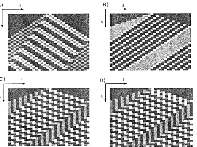
Fig.5.$\mathrm{A}-\mathrm{D}$ shows an instability of uniform flow of each models at the critical density.

Figure 5: Instability of Uniform flow in $\mathrm{A}$)$\mathrm{S}\mathrm{l}\mathrm{S}$ model $\mathrm{B}$)$\mathrm{E}\mathrm{B}\mathrm{C}\mathrm{A}2\mathrm{C}$)$\mathrm{E}\mathrm{B}\mathrm{c}\mathrm{A}1$

We can see the (

$‘ \mathrm{s}\mathrm{t}\mathrm{o}\mathrm{p}- \mathrm{a}\mathrm{n}\mathrm{d}-\mathrm{g}\mathrm{o}$

” _{wave propagates backward from the perturbated place}

of uniform flow in Fig.$5\mathrm{A},$ $\mathrm{C}$ and $\mathrm{D}$, i.e., the SIS model, the EBCAI model and the

SISEBCAI

model, respectively. The time evolution of the EBCAI and SISEBCAI model

show almost

same

pattern. This is explained as follows. The string “_{$\cdots 111020\cdots$ ”}

and

“ $\cdots 121212\cdots$ ” are _{both steady states} of _two models. These

are

represented at $\mathrm{B}$ and $\mathrm{C}$

in Fig.6, respectively.

Figure 6: Schematic fundamental diagram of EBCAI and SISEBCAI

If we add a perturbation to the state at $\mathrm{A}$, then the flow decreases and transits to the

state D. This is the case in Fig.5. In the lower branch $Q=-\rho+1$ of congested phase,

the string “ $\cdots 2222\cdots$” _{appears, while in the upper branch} $\mathrm{B}-\mathrm{C}$, the site $‘\prime 2$” is not last

more than two successive sites. We see in Fig.7 that ifa perturbation to the uniform flow

A is large enough, then the string “_{$\cdots 2222\cdot\cdot,$}” _{appears and direct transition from} A _to

$\mathrm{D}$

occurs.

5

Concluding

Discussions

In this paper, multi-value extension of the rule-184 family is studied. We conclude that

EBCAI model is good for traffic model. The S1S model is also good for trafficmodel, but

if we consider a higher speed model, then the difference between EBCAI and high speed

SIS

model($\mathrm{S}\mathrm{l}\mathrm{S}$-EBCAI) becomes little. We

can

easily deal

EBCAI

than the

S1S

model

because

EBCAI uses

only two successive time steps.

We investigate CAs’ with $L=2$, and only in the

case

ofEBCA2 we have commented

a result of general $L$. It is observed in other models with $L>3$ that there appear small

branches like those of EBCA2, but they have complicated nature than EBCA2. The

general results of the multi-value family and its two-dimensional extension will appear

elsewhere.

References

[1] H. Greenberg, Oper. Res., 7 (1959) pp.79.

[2] B. S. Kerner and P. Konh\"auser, Phys. Rev. E, 48 (1993) p.2335.

[3] G. F. Newell, Oper. Res., 9 (1961) p.209.

[4] M. Bando, K. Hasebe, A. Nakayama, A. Shibata and Y. Sugiyama, Phys. Rev. E. 51

(1995) p.1035.

[5] K. Nagel and M. Schreckenberg, J. Phys. I France 2 (1992) p.2221.

[6] M. Fukui and Y. Ishibashi, J. Phys. Soc. Jpn., 65 (1996) p.1868.

[7] D. E. Wolf, M. Schreckenberg and A. Bachem (editors), Workshop in

_Traffic

and

Granular Flow, (World Scientific, Singapore, 1996).

[8] S. Wolfram, Theory and Applications

_of

Cellular Automata (World Scientific,

Singa-pore, 1986).

[9] H. Fuk\’{s} and N. Boccara, Int.

J.

Mod. Phys. C, 9 (1998), p.1.

[11] Traffic Engineering (in Japanese), T. Sasaki and Y. Iida, Eds. (Kokumin Kagakusha., 1992).

[12] K. Nishinari and M. Hayashi (editors),

_Traffic

Statisticsin Tomei Express Way, (The

Mathematical Society ofTraffic Flow, Japan, 1999).

[13] R. Herman, E.W. Montroll, R.B. Potts and R.W. $\mathrm{R}\mathrm{o}\mathrm{t}\mathrm{h}\mathrm{e}\mathrm{r}\mathrm{y}\text{ノ}$. Opns. Res.,7 (1959) p.86.

[14] T. Tokihiro, D. Takahashi, J. Matsukidaira and J. Satsuma, Phys. Rev. Lett. 76

(1996) p.3247.

[15] K. Nishinari and D. Takahashi, J. Phys. A 31 (1998) p.5439.

[16] K. Nishinari and D. Takahashi, J. Phys. A 32 (1999) p.93.

Appendix

In this appendix, we will show a direct proof that a two-lane model of the rule-184 CA

corresponds to BCA with L $=2$. The two-lane model is shown in Fig.Al.

Figure Al: Two lane model of the rule-184 CA.

Cars move according to the rule-184 CA in each lane except the case of a lane change. If

a

car

exists in the site j in the A-lane and the site in front ofit is occupied, then the car

feel like changing its lane. When the site j and $j+1$ inthe $\mathrm{B}$-lane is empty, then the

car

will change its lane and go to the site $j+1$ in the $\mathrm{B}$-lane. This is the

same

changing rule

for a car in the $\mathrm{B}$-lane. Thus the lane change rule is represented by

$(A_{j}^{t}, A_{j1’}^{t}$$B_{j+1}+t)$

Bt,

$=$ (1, 1, 0,0) then $B_{j+1}^{t+1}=1$, $(A_{j}^{t}, A_{j+}^{t}B_{j}tB_{j}^{t})1"+1$ $=$ (0,0,1,1) then $A_{j+1}^{t+1}=1$.

Then time evolution of the A-lane is given by

$A_{j}^{t+1}$ $=$ $A_{j}^{t}+ \min(A_{j-1}t,1-A_{j}\iota)-\min(A_{j}t, 1-A_{j+}t)1$

$+ \min(1-A_{j1}^{t}-,1-AtBj’ j-1t, B^{t}j)-\min(A_{jj}^{t}.A^{t}1-+1’ B_{j}^{t}, 1-B_{j+}t)1’(10)$

where the first and second terms in right side hand of (10) represent the rule-184 $\mathrm{C}\mathrm{A}$,

and the third and fourth terms represent lane change of cars that come from and go to

the $\mathrm{B}$-lane, respectively. We replace $A$ to $B$, then we obtain time evolution for the B-lane

as

$B_{j}^{t+1}$ $=$ $B_{j}^{t}+ \min(B_{j-1}t,1-B_{j}t)-\min(Bjt, 1-B_{j+1}t)$

$+ \min(1-B_{j1}t1-\cdot-B^{t}, AtAjj-1’ jt)-\min(B_{j}^{t}, B_{j}t.1-A_{j}t1-A_{j}t)+1’+1$. (11)

Ifwe put

$U_{j}^{t}=A_{j}^{t}+B_{j}^{t}$, (12)

then summing (10) and (11), we can derive (1) with $L=2$ by simple calculations with

formulae $\min(A, B)+\min(A. 1-B)=A$ and $\min(A, B)+\min(c, D)=\min(A+C,$$A+$