SINGLE-MACHINE SCHEDULING WITH MIXED PRECEDENCE CONSTRAINTS

Vol. 42? No. 3? September 1999

SINGLE-MACHINE SCHEDULING

WITH MIXED PRECEDENCE CONSTRAINTS

Eugene Levner MiEan Vlmh

Center for Technoiog2cd Educat2on H o l m Japan Advaoced Instztute of Sc2ence and Technology

(Received July 8 7 1998; Revised January 29, 1999)

Abstmct The paper deals with a single machine scheduling problem involving a general precedence s t r ~ ~ c t u r e that permits both ordinary and fuzzy precedence constraints. Feasible schedules are evaluated not only by their cost but also by the degree of satisfaction with their precedence structure. An O ( m log n-i- max(n2, kn2))-time algorithm is proposed for finding no~dominated solutions of the resulting bi-criteria scheduling problem where n is the number of jobs, k is the number of fuzzy constraints> and m is the total number of precedence constraints.

1. Introduction

There are many s&eduling problems of practicd interest in which the input data are un- certain or imprecise, and their forms of uncertainty or imprecision are not of probabilistic nature. In situations where objective functions or constr&nts are neither deterministic nor ~robabilistic~ the problem may often be modelled with the help of fuzzy sets.

The aim of this paper is to study a scheduling problem involving both ordinary (crisp) and fuzzy precedence constraints. Machine scheduling problems with such constraints may occur in many different situations in modern automated systems. We now present several examples of such problems.

Consider a multi-machine robotic cell in which a robot (an automated guided vehicle) is responsible for loading/udoading and transporting parts between machines. The parts visit the machines according to given routing tables, thus generating demand for the robot. Various possible equipment layouts in such cells are presented, for example> in [l l2,l3]. The due dates of robot operations within a production cycle are specified by a process engi- neer, according to specific requirements of a production process. Further, the technologicd requirements impose that certain robot operations must precede some others. The deci- sion maker is faced with the problem of finding a robot's schedule subject to precedence constraints and minimizing some cost functian depending on completion times of robot o p e r a t i ~ ~ s .

Another example relates to a pick-and-place robot serving an automated warehouse. Suppose n items (orders) are waiting on their places in the warehouse for being sent to the customers. The pick-and-place robot has to serve them in turn, that is, to unload and transport them to the output one after mother. Due dates md unloading/transportation

times are known for each item. Some items may be unloaded only after some others, and these precedence constraints on robot's operations are specified in advance. Again, the decision maker is to find a schedule for the robot such that the precedence constraints are satisfied and a given function of operation completion times is minimized.

Consider a satellite following orbits around the Earth in order to take shots corresponding to images requested by various customers. One of the decision problems to be solved is the so-called daily task planning which consists in sequencing of tasks (shots) to be performed by the satellite during a planning period. Due dates and operation durations are known for each task. Precedence constraints between the tasks that range them according to their scientific, military, political or commercial importance are determined by experts and specified in advance. Since all the images requested cannot usually be satisfied in time, a penalty function is given for each task the value of which depends on time when the task is performed. In order to observe the interests of all customers, a shot sequence minimizing the maximum penalty (or some other function of penalties) is to be found. Often the quality of the resulting shot sequence must be evaluated by taking into account this criterion as well as the satisfaction of the decision maker with the task ordering.

In all examples given above, the precedence constraints may be crisp or fuzzy. The crisp precedence constraints describe the ordering between the operations which is not liable to any change under any circumstances (for example, it is a given technological order) while the fuzzy precedence constraints describe a more flexible situation where some pairs of operations are not linked by technological constraints but the decision maker prefers one ordering to another according to her or his intuition or experience. The choice of an order among these two possible alternatives for each pair of such operations is, in fact, a decision variable. As we shall see below, this choice may be carried out in such a way that the satisfaction of the decision maker with a schedule is maximized. The exact meaning of this criteria will be explained in the next section.

In the case when all precedence constraints are crisp, we obtain the classical single- machine n-job scheduling problem for which a great number of results is reported in the scheduling literature. Depending on the specific form of the objective functions and con- straints of the problem, many versions of the problem are known to be polynomially solvable while a lot of others are proved to be NP-hard (see, for example, the extensive survey [lO]). However, not too much is known about this scheduling problem when fuzzy precedence constraints are present.

Recently, Ishii and Tada [6] have addressed a single machine problem of minimizing max- imum lateness in the presence of fuzzy precedence constraints. They proposed an efficient combinatorial algorithm solving the problem in cubic time (with the problem size being measured in the number of jobs).

In this paper, we extend the above model in the following two aspects. Firstly, we deal with minimizing the maximum of arbitrary nondecreasing cost functions of completion times. Secondly, we consider a rather general precedence structure which includes both crisp and fuzzy precedence constraints.

Following the Ishii-Tada approach, we take the degree of satisfaction of the decision maker with respect to the precedence structure as the second criterion, and propose an

O(m log n

+

max(n2, kn2))-time algorithm for finding nondominated solutions of this bi- criteria scheduling problem, where n is the number of jobs, k is the number of fuzzy con- strains and rn is the total number of crisp and fuzzy precedence constraints.

In the next section we present the problem formulation. In Section 3 we present a new strongly polynomial algorithm for finding nondominated solutions of the resulting bi-criteria scheduling problem. In Section 4 we analyze the algorithm and obtain, as 'by-products', refinements of the Lawler and Ishii-Tada algorithms. Section 5 presents a numerical example. Section 6 summarizes the results of the paper and discusses some directions for further research.

2. Problem Formulation

We consider the following scheduling problem with mixed (crisp and fuzzy) precedence constraints.

1. There are n jobs Ji,

. . .

,

Jn to be processed on a continuously available machine which can execute at most one job at a time.

2. No preemption is permitted, i.e. each job Jj requires an uninterrupted processing time pj,

7

= 1,

.

. .

,

n, where all p j are positive rational numbers.

3. Two types of precedence constraints between the jobs are given:

(a) Crisp constraints that are specified in the form of a partial order given by an acyclic digraph G = (V, E), each node j E V corresponding to job Jj, and each arc (', k ) E E depicting that job Jj has to be completed before the processing of job Jk can start.

(b) Fuzzy constraints that impose that some pairs of jobs can be carried out in an arbitrary order but a certain order is more preferable than the opposite order,

om decision maker's point of view.

Thus, for each unordered pair of different jobs, Ji and Jj, exactly one of the following three mutually exclusive options occur: either (i) Ji and Jj are subject to a crisp constraint, or (ii)

Ji

and

4

are subject to a fuzzy constraint, or (iii) Ji and

Jj

are independent, that is, are related neither by a crisp nor by a fuzzy constraint.

Each fuzzy precedence constraint is specified by (i) an unordered pair of different jobs, = {J,,

J,}

and (ii) a membership function p u defined on the corresponding two- element set consisting of ordered pairs (Ji,

4 )

and (Jj, Ji). Here (Ji, Jj) denotes that Ji precedes J j a

To simplify the notation, we denote the two values of pu by pij and ki, that is,

( Ji, J j )

,

pji = p.

lJ,,

Ji)

.

The values {iij and

a,,

express the degrees of

on when job Ji precedes job Jj and when Jj precedes Ji, respectively. We a t each membership function

u,u

is normal and unirnodal, that is, one of the

j and /Èj is 1, and the other is strictly between 0 and 1.

with each job Jj is a nondecreasing cost function fj; if job Jj is completed cost fj(Cj) is incurred. Special cases of the general cost function are, for e lateness and tardiness.

the paper we denote the set {l, 2, . . .

,

n} of job indices by J and identify schedules with permutations of J . In other words, we are optimizing over the set chedules. We say that a permutation TT of J is compatible with a ose node-set is J, if, for each arc (2, j) from the transitive closure of

recedes

4

(not necessarily immediately) in permutation TT.

he quality of a schedule, we wish t o take into consideration not schedule but also the degree of satisfaction with the precedence dule. As a consequence, we obtain a bicriteria scheduling problem. minimize the maximum cost, and the other is t o maximize the with the job order. Since p 9 and pji are given for the define pij and pji for the remaining ordered pairs of

j = 1 and pji = 0 for each pair (2, j) belonging t o the transitive closure of the

precedence graph G;

For each permutation TT = ( ~ ( 1 ) ,7r(2),

. . .

,

v(n)) of {l, 2,

. .

.

,

n } that is compatible

wit h all crisp constraints, we define

where C j (T) denotes completion time of job J j under the permutation schedule given

by TT.

Since it may happen that no feasible schedule optimizes fmax and u,min simultaneously,

we are interested in finding schedules which are nondominated with respect to the following dominance relation: A schedule 71-1 is said to be dominated by a schedule

if

and at least one of these two inequalities is strict. If TT and TT' are such that

then we call them equivalent. Consequently, every equivalence class of schedules con-

sists of all schedules with identical value of fmax and identical value of Urnin.

Now the problem we are addressing in this paper can be formulated in the following way.

Problem P: Find one schedule from each equivalence class of nondominated

feasible schedules.

Let us note that this problem includes several known scheduling problems as special cases. For example:

(a) In the case that only crisp precedence relation is imposed, the above problem reduces t o the Lawler single-machine scheduling problem [g].

(b) If the set of crisp precedence constraints is empty, and each cost function f j is the lateness with respect t o a given due date d j that is, /,(Cj) = Cj

-

d j , then the above problem reduces to the Ishii-Tada problem with fuzzy precedence relation [6].

( c ) If precedence relations (both crisp and fuzzy) are absent and functions f j are specified as membership functions measuring the degree of expert's dissatisfaction, then the problem becomes a scheduling problem with fuzzy due dates (see, for example, Ishii et al.[7], Han et al. [5], Tanaka and Vlach [14], and Vlach [15]).

3. Problem Analysis and Algorithm

In what follows,

Ga

stands for a digraph defined for each 0

< a

5

1 as follows: If a = 1, then

Ga

=

Gl

is the digraph obtained from the crisp precedence graph G by adding to it all arcs (I, j) corresponding to the fuzzy constraints with b j = 1. If 0

<

a

<

l, then

Ga

is the digraph obtained from Gl by deleting all arcs (i, j) such that pi, = 1 and

>

a. After this deletion, there remain only arcs ( i , j ) with p,, = 1 and / ^ j i

<

a in the resulting

graph. Note that graph Ga may contain directed cycles for some values of a.

For ease of description of solution procedures for problem P, we consider also the fol- lowing auxiliary problems Pa, 0 < o.

<

1:

Minimize jmax (T) subject to p 4

>

a,

TT is compatible with

Go,.

As pointed out in the previous section, Ishii and Tada [6] proposed an O(n3)-time al- gorithm for solving problem P in the case that no crisp constraints are present, graph

Gi

is acyclic, and fm is the maximum lateness. For reader's convenience we recall the basic steps of their algorithm.

THE ISHII-TADA ALGORITHM

[Initialization]

.1 Arrange all / i i j from the open interval ( 0 , l ) in nondecreasing order and rename the

resulting

k

different values so that

1.2 Set q := 0, p(q) := 1, a := p(q), L :=

0.

1.3 Construct

Ga

as described above.

Step 2 [Solving

Pal

Minimize the maximum lateness subject to the precedence relation given by

Ga.

If the resulting solution is not dominated by any schedule from L

and TT& is not yet in L, then include it in L.

Step 3 [Arc deletion] If q < k , then set q := q

+

1, a := p(q), construct

Ga

by deleting from Gp(n-n all arcs (i, j) with pj; = a, and go to Step 2. If q = k, then stop (the current L provides the required set of nondominated solutions).

The extension of the Ishii-Tada approach to the general case proposed in this paper is based on the following four observations.

Observation 1 Solution of problem

Pa

in the second step of the Ishii-Tada algorithm can be implemented in polynomial time not only for the maximum lateness but also for an arbitrary function fmã defined by (2), provided all

f,

are nondecreasing and their values

can be computed in constant time.

Proof. The well known algorithm of Lawler [g] provides the required possibility. To obtain a concise description of this algorithm we use the following notation. Let the precedence relation under consideration be given by an acyclic digraph G = (V, E). Without loss of generality we assume that V is the set of the job indices {l, 2,

. . .

,

n}. For each subset I of

V, let be the digraph obtained by restricting G to I. Furthermore, for each 2 E I, let

%(GI) denote the set of all nodes in I preceded (not necessarily immediately) by node 2,

and let Ei(GJ) denote the set of all arcs of GI entering node i. Now we are ready to describe the algorithm.

THE LAWLER ALGORITHM

I:=

V,

A:=E,

M :=

EiEI

pi

For j = n down t o 1 do: Choose 2 6 I such that

/ $ ( U ) = m i n { j ~ ~ I~,.(G~)=O~ /.(U)

I:=

1

\

{i}, A := A

\

Ei(GI) u : = u - p i

~ ( j ) := 2

The algorithm determines the index v(>) of the job in the i-th position of an optimal permutation schedule, and the analysis presented in [g] shows that the algorithm can be run in 0(n2)-time. D

Observation 2 If graph Go contains a cycle, then problem P has no feasible solution v with p i m d

>

a.

Proof (by contradiction). Assume that problem P has a feasible solution v with pmin(v)

2

a, and that graph Go has a directed cycle C. Rename the nodes of V so that v = (1,2,.

.

.

,

n).

Let C = (vl, v2,.

.

.

,

vti vl) where

t

<

n. Let U denote the smallest node in C, and W the

node standing just before U in C. [For instance, if v = (1,2,3,4,5,6) and C = (6,5,3,6)

then U = 3 and W = 51. Consider two possible cases.

CASE A. Suppose that arc (W, U) of C (in graph Go) corresponds t o a crisp constraint. According to the definition of the crisp constraint, it means that job Jw must precede job Ju in all feasible schedules. On the other hand, any feasible permutation (and v as well) determines uniquely an order of processing the jobs. Since, in accordance with our choice,

U

<

W in v, then Ju is to be processed before Jw in schedule v. This condition, taken

together with the above one that Jw precedes Ju, contradicts our basic assumption that the crisp precedence graph G =

(V,

E) is acyclic.

CASE B. Arc (W, U) in Go corresponds to a fuzzy constraint.

According to the construction of Gl and Go, p"wu = 1. However, Ju precedes Jw in

v (because of U

<

W). Therefore, pã will be participating in defining the value pmin(v)

according to (1). Recall now that graph Go is constructed by deleting from Gl all arcs with pji

>

a, leaving only those (i, j ) for which

<

a . Then pmiii(r) < a, which contradicts the assumption that pmin(7i")

>

a. This proves the claim.

a

Observation 3 If graph GB contains a cycle for some 0

< /?

5

1, then the maximum value of a in the interval 0 < a <

/?

for which Go is acyclic can be found by a binary search.

Proof. First we notice that if problems Pol and

Pm

with 0 < a1

<

<

Q

are such that the

corresponding graphs Gal and Gm have cycles, then also the graph Go corresponding to

Pa

contains a cycle whenever 0

<

a1

<

a

<

a^. This is obvious because Gm is a subgraph

of Go for each 0

<

a-\

< a

<

Q.

It remains to show that there exists a in the interval (0, Q) such that Go is acyclic. According to the assumption, graph GÃ contains a cycle. It follows that GP contains arcs corresponding to fuzzy constraints, because the graph defining the crisp constraints is assumed t o be acyclic. It follows, also from the acyclicity of the crisp precedence, that we can obtain an acyclic graph Go with 0

<

a

<

Q by deleting from Go sufficiently many arcs corresponding to fuzzy constraints. Now, if graph GP contains a cycle we can arrange all k j values from ( 0 , l ) corresponding to its fuzzy constraints in

decreasing order. Obviously the number of different pq values is not greater than m, the total number of all precedence constraints. Since graph G is an acyclic subgraph of GP, the standard binary search will identify the maximal / ~ y for which the graph Gpij is also acyclic

in O(1og n) time. D

Observation 4 If GP is acyclic for some 0

<

,B

<

1, then there is a generalization of the arc deletion procedure of the third step of the Ishii-Tada algorithm such that it can be applied for a transition from PÃ to Pa with 0 < a

<

p.

Proof. Consider an arbitrary feasible schedule v for problem Pa with 0

<

a

<

Q. Let jobs

Ji and Jj be such that

the arc ( Q ) belongs to GP,

If job Ji is scheduled before job Jj in v, then there are k and Z such that

If job Ji is scheduled after job Jj in v , then there are k and l such that

I t follows that in both cases , ~ ~ ( k ) ~ ( i )

2

a. However, as Ishii and Tada noticed in [6], this

implies that an arc (2, j ) can be discarded from Go without violating the feasibility condition k i n ( r )

>

a. Moreover, the minimum of fmnE subject to the precedence constraints given by GP

\

{(i, j ) } cannot be smaller than the minimum of

fmia

subject t o GB, because GB

\

{(i, j)} is a subgraph of GB. This argument can be repeated iteratively for all arcs (i, j) of GB for which pu = 1 and

u,a

>

a, as required by the Ishii-Tada arc deletion procedure. D

Algorit hm Description Step 1 [Initialization]

1.1 Arrange all p;, from the open interval ( 0 , l ) in nondecreasing order and rename the resulting k different values so that

1.2 Set q := 0, p(q) := 1, a := pi(q), L :=

0.

1.3 Construct Ga by adding to the crisp precedence graph all arcs (i, j) corresponding t o the fuzzy constraints with /^j = 1.

Step 2. Check if graph Ga is acyclic. If yes, go t o Step 4; if no, go to Step 3.

Step 3. [Binary search] Find i such that p(i) is the greatest value among /((I),

.

. .

,

li(k)

such that the corresponding graph Gain is acyclic. Set a := p(+

Step 4. [Solving Pal Solve problem Pa- If the resulting solution ra is not dominated by any schedule from L and G is not yet in L, then include it in L.

Step 5 [Arc deletion] If q

<

k , then set q := q + 1, a := p(q), construct Ga by deleting from Gp(q-i) all arcs (i, j) with fi,. = p(q - l), and go to Step 4. If q = k, then stop

(the current L provides the required set of nondominated solutions).

4. Analysis of the Algorithm

In what follows we will assume, without loss of generality, that all fuzzy arcs have different membership function values. If some arcs have identical pij values, for example, p ( l ) = p(2) =

. . .

= p ( d ) , then we let p'(i) = p(i)

+

€ for i = 1,

. .

.

,

d, where e

>

0 is a small

number and we use ei to break ties.

Theorem T h e time complexity of the algorithm i s O(m log n

+

max(n2, kn2)) where k is the

number of fuzzy constraints, m is the total number of precedence constraints, and n is the

number of jobs. Proof.

Step 1.1 requires 0 ( k log n) operations.

Step 1.2 and Step 1.3 can be run in 0 ( m ) time.

Step 2 can be done in 0 ( m ) time (see, for example [2]).

Step 4 requires 0 ( n 2 ) , according to the complexity of the Lawler algorithm [g] when the

scheduling problem is solved from scratch. Then this step is repeated a t most k

+

1 times, each time requiring 0 ( n 2 ) operations. Thus the total time for this step is 0(kn2).

Step 5 requires at most 0 ( m ) time.

Thus, the overall time complexity of the algorithm is O(m log n

+

max(n2, An2)).

a

Corollary 1. (Refinement of the Lawler-Moore algorithm for Lam)- The time complexity of minimizing the maximum lateness subject t o crisp precedence only is O(m

+

n log n). Proof. Note that 0 ( m ) time is needed to construct graph TG, the topologically sorted representation of the directed acyclic graph G [2]. Let 1,2,

. . .

,

n be the new numbers of nodes of G, linearly ordered in TG.

According to the Lawler-Moore algorithm [l11 for minimizing the maximum lateness

Laax = maxj(CJ - dj), we need to determine and sort the modified due dates:

where Tj is the set of all successors (not necessarily immediate) of j in TG.

Let Wj be the set of immediate successors of j in TG and Nj be the number of nodes in Wj. Since T G is topologically sorted, we can rewrite the definition of d$ as follows:

Let us calculate dk, d L l ,

. .

.

,

di in this order. In order to know dk we now need O(1) time. Further, in order t o know d l we need O(Nn-1) operations, to know dk-, we need O(Nn-2) operations, and so on, till we find d', using O(Nl) operations.

The total time is O(Nl

+

+

Nne1) = 0(m).

To sort the d',, we need O(n log n) time, and this proves the claim. U

The estimation refines the Lawler-Moore result [l11 in practically important cases when m is less than n2, and coincides with it in the case when m is close to n2, for example, if G is complete.

Corollary 2. (Refinement of the Ishii-Tada algorithm). If Gi is an acyclic digraph in

which the maximal distance between pairs of its nodes is H, then the algorithm can be run in O(m logn

+

Hk) time.

Proof. When applying the above algorithm t o the Ishii-Tada problem, Steps 2 and 3 are not exploited, while Step 4 requires now only 0 ( m ) operations when the problem is solved from scratch. In addition, 0 ( H k ) time is needed, because 0(H) operations are applied to recalculate the modified due dates, the latter recalculations being repeated 0 ( k ) times, each time for a new problem

Pa.

D

The estimation refines the Ishii-Tada result in [6] when m is less than n2, and coincides with it when m is 0(n2). As an obvious consequence of this corollary, we obtain the following result.

Corollary 3. ( The case of planar graphs). If, in addition to the assumption of the previous Corollary, the precedence graph is planar, then the problem can be solved in 0 (nlog n

+

H n )

time.

5. Example

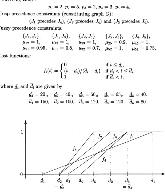
Processing times:

Crisp precedence constraints (constituting graph G):

( Jl precedes J4), ( J 2 precedes J4) and (Ja precedes J4).

Fuzzy precedence constraints:

Cost functions:

where

di

and

di

are given by

d l = 2 0 , , d 2 = 4 0 , , & = 5 0 , , & = 6 5 , , & = 4 0 . -

- -

dl = 150,

d2

= 100,

d3

= 120, d4 = 120, d5 = 80.

Figure 1: Cost functions

Obviously these cost functions (see Figure 1) can be interpreted as fuzzy due dates which describe the degree of dissatisfaction of a decision maker with job completion times as follows. The decision maker is completely satisfied (his degree of dissatisfaction is zero) when job Ji is completed by time cli, and his degree of dissatisfaction increases linearly as the job completion time increases, achieving the maximal value 1, if the job is completed at or after

di

(see for example [5,7,14,15]).

The proposed algorithm works as follows.

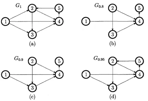
Step 1: We obtain k = 5 and

where p(1) = b1=0.95; p(2) = p25 = 0.9; p(3) = pal = 0.8; p(4) = pst = 0.75 and

Step 2: It turns out that graph Gl contains a cycle. Thus, we must go t o Step 3.

Step 3: Step 3 is performed in three iterations.

In the first iteration, we find that graph Goa is acyclic. In the second iteration, we find that graph Gomg is also acyclic. Finally in the third iteration, we find that Go.95

has a cycle. After the third iteration we go to Step 4.

Step

4:

Step

4

is performed sequentially four times, for a = 0.9,0.8,0.75 and 0.7, respec- tively (see Figure 3).

Figure 2: Binary search of an acyclic graph

At each iteration of Step 4, the corresponding problem

Pa

is solved with the help of Lawler's algorithm. The corresponding solutions are:

if a = 0.9 then 71-1 = (l, 2,3,4,5) with fnia(ri) = 1 and _/imin(r1) = 0.9; i f a = 0 . 8 t h e n m = ( 2 , 3 , 1 , 4 , 5 ) w i t h f m a x ( ~ 2 ) = 1 and/imin(%)=0.8; if a = 0.75 then = (5,2,3,1,4) with f m v . ( ~ ) = 0.3 and = 0.75;

if a = 0.7 then 71-4 = (5,3,2,1,4) with

fma(r4)

= 0.25 and pmin(r4) = 0.7.

Notice that schedule 7r2 is discarded at Step 4 because it is dominated by schedule 71-1.

Three remaining schedules constitute the set of nondominated solutions, for this example.

6. Concluding Remarks

This paper introduces a new practically important class of one-machine scheduling prob- lems, the so-called problems with mixed precedence constraints, which include both crisp and fuzzy precedences. It is shown that the two types of precedences not only have dif- ferent physical nature but also require a different algorithmic treatment in the scheduling problems. The scheduling problem under consideration is formulated as a bi-criteria combi- natorial optimization problem, and a set of nondominated solutions is obtained in strongly polynomial time. Examples of applications in robotic automated systems are presented.

Several extensions of this study may be of practical value. First, it is certainly possible that the polynomial algorithm presented in this work can be further improved.

Figure 3: Solution process

Another extension is concerned with applying the suggested approach for fuzzy schedul- ing in wider practice-oriented directions: (a) more than one machine may be treated with other criteria and scheduling scenarios, like job shop, open shop, cyclic shop or general shop, (b) other types of fuzzy constraints and fuzzy input data could be involved, (c) synchro- nization and coordinated scheduling of machines and automated material-handling devices

(robots) in flexible manufacturing systems are of special interest.

Acknowledgments

This work was performed while the first author was visiting the Japan Advanced Institute of Science and Technology, Ishikawa. The support of this author by the International In- formation Science Foundation (grant 97.1.3.615) and by the Ministry of Science of Israel in the framework of the cooperative program with the Japan Society for the Promotion of Science (grant 8951.1.97) is gratefully acknowledged. The authors thank J.K. Lenstra for a very helpful comment.

References

J.L. Cheng, H. Kise, and Y. Karuno: Optimal scheduling for an automated m-machine flowshop. Journal of Operations Research Society of Japan, 40-3 (1997) 1-15.

T.H. Cormen, C.E. Leiserson, and R.L. Rivest: Introduction to Algorithms (The MIT Press, Cambridge, 1990).

C. Gaspin: Mission scheduling. Telematics and Informatics, 6 (1989) 159-169.

N.G. Hall and M. J. Magazine: Maximizing the value of a space mission. European Jour- nal of Operational Research, 78 (1994) 224-241.

S. Han, H. Ishii, and S. Fujii: One machine scheduling problem with fuzzy duedates. European Journal of Operational Research, 79 (1994) 1-12.

.

Ishii and M. Tada: Single machine scheduling problem with fuzzy precedence relation. European Journal of Operational Research, 87 (1995) 284-288.

[7] H. Ishii, M. Tada, and T. Masuda: Two scheduling problems with fuzzy due-dates. Fuzzy Sets and Systems, 46 (1992) 339-347.

[8] H. Kise, T.Shioyama, and T. Ibaraki: Automated two-machine flowshop scheduling: a solvable case. IIE Trans., 23 (1991) 10-16.

[g] E.L. Lawler: Optimal sequencing of a single machine subject to precedence constraints.

Management Science, 19 (1973) 544-546.

[l01 E.L. Lawler, J.K. Lenstra, A.H.G. Rinnooy Kan, and D.B. Shmoys: Sequencing and scheduling: Algorithms and complexity. In S.Graves, A. Rinnooy Kan and P. Zipkin (eds.): Logistics of Production and Inventory, Handbooks in Operations Research and Management Science (Elsevier, New York, 1993), Vol.4, 445-522.

[l11 E.L. Lawler and J.M. Moore: A functional equation and its application to resource allocation and scheduling problems. Management Science, 16 (1969) 77-84.

[l21 Y.H. Pao and M. Jelinek: Flexible Manufacturing Cells and Systems. In R.C. Dorf and S.Y. Nof (eds.): International Encyclopedia of Robots: Application and Automation

(Wiley, New York, 1988), 530-551.

[l31 E. Levner, K. Kogan, and I. Levin: Scheduling a two-machine robotic cell: A solvable case. Annals of Operations Research, 57 (1995) 217-232.

[l41 K.Tanaka and M.Vlach: Single machine scheduling with fuzzy due dates. In: Pro- ceedings of the VII International Fuzzy Systems Association World Congress, IFSAJ97

(Academia, Prague, 1997), Vol. I, 30-35.

[l51 M. Vlach: Scheduling and sequencing in a fuzzy environment. In: Proceedings of the VII International Fuzzy Systems Association World Congress, IFSA '97 (Academia, Prague,

1997), Vol. Ill, 195-199.

Milan Vlach

School of Information Science,

Japan Advanced Institute of Science and Technology, 1-1 Asahidai, Tatsunokuchi, Ishikawa 923-1292, Japan. E-mail: vlach@ jaist

.

a c

.

j p