2008, Vol. 51, No. 3, 225-240
OPTIMAL TIME TO INVEST UNDER UNCERTAINTY WITH A SCALE CHANGE
Naoki Makimoto University of Tsukuba
(Received November 7, 2006; Revised April 4, 2008)
Abstract In this paper, we investigate the optimal investment problem to maximize expected discounted payoff of a project whose value is given by a product of two processes: a geometric Brownian motion representing continuous fluctuation over time and a Markov process which gives a discontinuous scale change. It turns out that the optimal policy is of threshold type whose thresholds depend on the current state of the Markov process. For 2-state case, the problem can be solved explicitly by using Bellman equation and smooth pasting conditions. On the other hand, the problem becomes much involved when there are multiple states. We exploit the structure of the optimal policy and the form of the value functions which enables us to develop a simple numerical procedure for computing the optimal policy and the value functions.
Keywords: Finance, optimal investment, stopping problem, Bellman equation, smooth pasting
1. Introduction
Recently, many papers have studied optimal investment problems under uncertainty. The main objective of these researches is to find optimal time to invest so as to maximize the expected future payoff under the assumptions on the stochastic dynamics of the project value, investment opportunity, investment cost, and so on. In contrast to the traditional approaches for valuing projects, these analyses makes it possible to explicitly incorporating such flexibilities as option to invest, defer and expansion into decision making. As a result, a variety of models have been analysed and applied to practical problems in the context of real option analysis [12].
The basic form of the optimal investment problem is to maximize expected discounted payoff of the project with a constant investment cost. Assuming that the project value follows a geometric Brownian motion, the optimal policy is shown to be of threshold type and the value function and the optimal threshold are explicitly obtained. Since the seminal book by Dixit and Pindyck [3], this basic problem has been extended in many directions. D´ecamps et al. [2] analyses a problem in which an investor has to choose among two alternative projects with different characteristics. Guo [5] and Guo et al. [6] introduce Markovian regime shifts into the drift and volatility of a geometric Brownian motion. Ohnishi and Tsujimura [10] considers an optimal investment problem with transaction costs. Vollert [13] discusses several types of optimal investment problem in a stochastic control framework.
In this paper, we investigate the optimal investment problem in which the project value is given by a product of two processes. One process follows a geometric Brownian motion which represents continuous fluctuation over time as in the most previous studies. Another source of uncertainty is given by a Markov process which gives a discontinuous scale change
to the project value. From practical point of view, such a scale change will be caused, for example, by preemption or exit of other companies, drastic changes of product price, and so on. We first show that the optimal policy is of threshold type whose thresholds depend on the current state of the Markov process. By using the standard approach based on Bellman equation and smooth pasting conditions, the optimal solutions can be obtained explicitly for 2-state case. On the other hand, the structure of the optimal policy becomes much involved when there are multiple states. We therefore exploit the structure of the optimal policy and the form of the value functions which enables us to develop a simple numerical procedure for computing the optimal policy and the value functions.
This paper is organized as follows. In Section 2, we formulate the optimal investment problem. In Section 3, we investigate the characteristics of the optimal policy. Section 4 is devoted to solving Bellman equation to identify the form of the value functions. Finally in Section 5, we consider some computational issues and show some numerical examples. 2. The Optimal Investment Problem and Preliminary Results
In this section, we describe an investment decision problem and formulate it as an opti-mization problem. Suppose there is a project to which we are going to invest some amount of money. At any time point until investment has been executed, we can choose either to invest now or to wait for future investment. If we decide to invest at t, then we will receive payoff Vt− I where Vt is a value of the project and I is an investment cost.
In this paper, we assume that the project value is given by Vt= StUt. Conceptually, Ut represents the continuous fluctuation over time and St gives a discontinuous scale change or multipilcative shock to the project value. As in standard real option models, we assume that {Ut} follows a geometric Brownian motion:
dUt
Ut
= µdt + σdzt (2.1)
where drift µ and volatility σ are constant and {zt} is a standard Brownian motion. It is well known that the solution of Equation (2.1) is given as a geometric Brownian motion:
Ut= U0exp{(µ − σ2/2)t + σzt}. (2.2)
On the other hand, {St} is a continuous-time Markov process on the state space S =
{s1, . . . , sN} governed by the transition rate matrix Q. Throughout the paper, we assume without loss of generality 0 < s1 < s2 < · · · < sN < ∞. We also assume that {Ut} and
{St} are mutually independent. A constant investment cost I is incurred at the time of investment and a future payoff is discounted by an exogenously given discount rate ρ, as in the most literatures on real option analysis. To assure the existence of the expectation, we assume ρ > µ.
The investment decision problem can be formulated as
Fi(u) = sup τ≥0
E[e−ρτ(SτUτ − I)|S0 = si, U0 = u] = sup τ≥0
Ei,u[e−ρτ(SτUτ − I)]. (2.3) The supremum is taken over all stopping times with respect to the filtration generated by
{Ut} and {St}. Here and in what follows, we use the abbreviated notation Ei,u[ · ] instead of E[ · |S0 = si, U0 = u] for notational simplicity.
For later use, we introduce the optimal solution when St= s is a constant. The problem in this case is to obtain
H(u; s) = sup
τ≥0
(we specify the dependence of H(u; s) on s). Then, as described in Dixit and Pindyck [3], the optimal policy is to invest at the first time Ut≥ υ occurs and the value function under this policy is given by
H(u; s) = (sυ− I υξ ) uξ, 0 < u < υ, su− I, u≥ υ (2.5) where υ = ξI (ξ− 1)s, ξ = f +(ρ) > 1.
In the sequel, we use the notations
f+(a) = σ 2/2− µ +√(σ2/2− µ)2+ 2σ2a σ2 (> 1,∀a > 0), (2.6) f−(a) = σ 2/2− µ −√(σ2/2− µ)2 + 2σ2a σ2 (< 0,∀a > 0) (2.7) to represent the solutions of a quadratic equation
σ2
2 x 2− (σ
2
2 − µ)x − a = 0.
Remark 2.1 In real option analysis, it is common to define the objective function (2.3) by sup
τ≥0Ei,u[e
−ρτmax(S
τUτ − I, 0)] (2.8)
to clarify the analogy with financial call options [3]. It is however obvious that Equations (2.3) and (2.8) lead to the same value function and optimal investment time since it is never optimal to invest when StUt < I and, starting with any initial values of S0 ∈ S and U0 > 0,
StUt> I occurs at some future time t with probability 1.
Before closing this section, we state the following result whose proof can be found in a standard textbook on differential equations.
Lemma 2.1 For a≥ 0, the solution of the ordinary differential equation
−ag(u) + µug′(u) + σ2 2 u 2g′′(u) + bu + c = 0 (2.9) is given by g(u) = d1uξ1 + d2uξ2 + b a− µu + c a where ξ1 = f+(a) > 1, ξ2 = f−(a) < 0. Coefficients d1, d2 should be determined by boundary conditions.
3. Characterization of the Optimal Policy
In this section, we investigate the characteristics of the optimal investment policy. The next lemma indicates that the optimality of threshold policy for the problem (2.4) is inherited even when St is stochastic. Optimal policy of threshold type can be found in a variety of investment problems [2, 3, 5, 6, 10, 13].
Lemma 3.1 The optimal investment policy is of threshold type, i.e., corresponding to the state of St, there exists a threshold υi (i = 1, . . . , N ) such that it is optimal to invest at time t if St= si and Ut ≥ υi, and it is optimal to continue waiting otherwise.
(Proof) Fix S0 = si. Suppose to the contrary that there exist u < ˜u such that it is optimal to invest when U0 = u while waiting is optimal when U0 = ˜u. From Equation (2.2), we can define Ut = uexp{(µ − σ2/2)t + σzt} and ˜Ut = ˜uexp{(µ − σ2/2)t + σzt} by the same Brownian motion {zt}. From the assumption, we have
siu− I ≥ Ei,u[e−ρτ(SτUτ − I)] (3.1)
for any {Ft}-stopping time τ, and
siu˜− I < Ei,˜u[e−ρ˜τ(Sτ˜U˜τ˜− I)] (3.2) where ˜τ is the optimal stopping time for{ ˜Ut}. If one uses the policy to invest at ˜τ for {Ut}, we obtain from u < ˜u that
e−ρ˜τ(S˜τUτ˜− I) = e−ρ˜τ( u ˜ uSτ˜U˜˜τ− I) > u ˜ ue −ρ˜τ(S ˜ τU˜τ˜− I) − (1 − u ˜ u)I. (3.3)
By taking the expectation on both sides of Equation (3.3) and using Equation (3.2), we get
Ei,u[e−ρ˜τ(Sτ˜Uτ˜− I)] > u ˜ uEi,˜u[e −ρ˜τ(S ˜ τU˜τ˜− I)] − (1 − u ˜ u)I > u ˜ u(siu˜− I) − (1 − u ˜ u)I = siu− I. (3.4)
Since the inequality (3.4) contradicts the fact that (3.1) holds for any τ , this completes the
proof. 2
Since the project value Vt = StUtchanges discontinuously when Sttransits from one state to another, an investment will be executed at the time either Utreaches the threshold υi from below while St = si remains unchanged, or St transits from si to si+1 when υi+1≤ Ut< υi.
From Lemma 3.1, we see
Fi(u) > siu− I, 0 < u < υi,
Fi(u) = siu− I, u≥ υi.
If υi < ∞, Fi(u) connects to the straight line siu − I from above at u = υi. It should be noted that some of υi may be infinite which means it is never optimal to invest when
St= si. However, at least υN <∞ as shown in the next lemma. Lemma 3.2 υN < υ1 and υN <∞.
(Proof) If s1 =· · · = sN = s, all value functions must equal H(u; s). Since s1 < s2 <· · · <
sN, we therefore obtain
Notice that the graph of H(u; s) connects from above to the straight line su−I at u = (ξ−1)sξI [3]. Since Fi(u)≥ siu− I for all u > 0, it is clear that (ξ−1)sξI 1 ≤ υ1 and υN ≤ (ξ−1)sξI N must hold so as to satisfy (3.5). The result follows since (ξ−1)sξI
N <
ξI
(ξ−1)s1 <∞. 2
When {St} has only two states, we see υ2 < υ1 from Lemma 3.2. However, the order of υi’s is not automatically determined when there are more than two states. In general, there seems to exist no simple way to identify the order of υi’s. This makes the problem of solving Bellman equation to obtain the value functions much involved.
In what follows, we provide a simple and useful condition to assure υN ≤ · · · ≤ υ1. Let
St(i) denote the conditional process of St starting with S0 = si.
Theorem 3.1 If one can construct sample paths of {St(i)} and {St(i+1)} on the same prob-ability space so as to satisfy
P (St(i+1)− St(i) ≤ si+1− si, ∀t ≥ 0) = 1, (3.6) then υi+1 ≤ υi.
The meaning of the condition in Theorem 3.1 seems unclear at first sight. Before proving the theorem, we give an illustrative example which satisfies the condition.
Example 3.1 Suppose that {St} follows a birth-death process with the transition rate matrix Q = −α1 α1 O β2 −(α2+ β2) . .. . .. . .. . .. . .. −(αN−1+ βN−1) αN−1 O βN −βN
and the state space is composed of N equally spaced states with unit interval s, i.e., sk =
s1+ (k− 1)s for k = 2, . . . , N. If the transition rates satisfy
α1 ≥ α2 ≥ · · · ≥ αN−1, β2 ≤ β3 ≤ · · · ≤ βN, (3.7)
then the condition in Theorem 3.1 is satisfied for all i = 1, . . . , N − 1 as we will see below. The condition (3.7) implies that the lower (higher, respectively) the current state is, the more likely the process will move to higher (lower) state. This property is so called mean reversion which is observed in a variety of financial time series such as interest rate and price of commodities.
To see that the condition (3.7) implies that in Theorem 3.1, let P = I + Q/θ be a transition probability matrix obtained by uniformization where θ = max1≤k≤N{αk+ βk}. Denote by {Sn} a discrete time Markov chain governed by P and let {N(t)} be a Poisson process with intensity θ which is independent of{Sn} and {zt}t≥0. The subordinated process
St= SN (t)is a continuous time Markov chain governed by Q (see Example 4.2 of Kijima [7]). Let Y1, Y2, . . . be a sequence of independent uniform random variables which is independent of {N(t)}. We construct the conditional process {S(j)n } starting with sj by setting S
(j) 0 = sj and S(j)n+1= sk− s, Yn+1 < βk/θ, sk, βk/θ ≤ Yn+1 < 1− αk/θ, sk+ s, 1− αk/θ ≤ Yn+1 (3.8)
when S(j)n = sk. Here we use the convention αN = β1 = 0. If we generate sample paths of
{S(i)
n } and {S (i+1)
that S(i+1)n − S(i)n ≤ si+1− si,∀n = 0, 1, . . .. By setting St(j) = S (j)
N (t) for j = i, i + 1, we can construct sample paths of {St(i)} and {S
(i+1)
t } which satisfy Equation (3.6). Now we prove Theorem 3.1.
(Proof of Theorem 3.1) Suppose to the contrary that υi < υi+1 and choose arbitrary u ∈ (υi, υi+1). Let ˜τ be the optimal investment time starting with S0 = si+1 and U0 = u. From the choices of u and ˜τ , we have
Fi(u) = siu− I > Ei,u[e−ρ˜τ(S (i) ˜
τ Uτ˜− I)], (3.9)
Fi+1(u) = Ei+1,u[e−ρ˜τ(S˜τ(i+1)Uτ˜− I)] > si+1u− I. (3.10) By the assumption of Theorem 3.1, we can obtain
e−ρ˜τ(S˜τ(i+1)Uτ˜− I) − e−ρ˜τ(S (i) ˜
τ Uτ˜− I) ≤ e−ρ˜τ(si+1− si)U˜τ (3.11) for any sample path of{Ut} independently chosen from {St(j)} (j = i, i+1) and for resulting sample of ˜τ determined by{St(i+1)} and {Ut}. Then,
Fi+1(u) = Ei+1,u[e−ρ˜τ(S (i+1) ˜ τ Uτ˜− I)] ≤ Ei,u[e−ρ˜τ(S (i) ˜
τ U˜τ − I)] + (si+1− si)Ei+1,u[e−ρ˜τU˜τ] (3.12)
< siu− I + (si+1− si)u (3.13)
= si+1u− I. (3.14)
Inequality (3.12) follows by taking expectation of (3.11) with respect to the independent probability measures on{St(j)} and {Ut}. To show inequality (3.13), note that
u≥ Ei+1,u[e−ρ min(˜τ,T )Umin(˜τ ,T )]≥ Ei+1,u[e−ρ˜τUτ˜1{˜τ≤T }] (3.15) holds for all T > 0 where 1A is an indicator function of A. The first inequality in (3.15) follows from optional sampling theorem applied to supermartingale{e−ρtUt} and the second one follows from Ut > 0. Since P (˜τ < ∞) = 1, we obtain from monotone convergence
theorem lim T→∞Ei+1,u[e −ρ˜τU ˜ τ1{˜τ≤T }] = Ei+1,u[e−ρ˜τU˜τ] (3.16) which together with inequalities (3.9) and (3.15) prove (3.13). Since inequality (3.14)
con-tradicts (3.10), the proof is completed. 2
In addition to the order of υi’s, we need to know whether υi <∞ or not to solve Bellman equation. To this end, let Sk={sk+1, sk+2, . . . , sN} and let κik be the first passage time of
St from si intoSk. Now suppose S0 = si and U0 = u and consider the following policy: (a) invest at κik irrespective of the value of Uκik.
Denote by Gik(u) the expected payoff of policy (a). Since {St} and {Ut} are assumed to be independent, Gik(u) is calculated as
Gik(u) = N
∑
j=k+1
Ei,u[e−ρκik(sjUκik − I)1{Sκik=sj}]
= N ∑ j=k+1 ∫ ∞ 0 e−ρtEi,u[sjUt− I]P (κik ≤ dt, St= sj) = N ∑ j=k+1 ∫ ∞ 0 e−ρt(sjueµt− I)P (κik ≤ dt, St= sj) = N ∑ j=k+1 [ fij(k)(ρ− µ)sju− f (k) ij (ρ)I ] (3.17)
where
fij(k)(s) =
∫ ∞
0
e−stP (κik ≤ dt, St = sj) = E[e−sκik1{Sκik=sj}]. (3.18)
fij(k)(s) can be calculated as follows. Let Q(k)1 and Q(k)2 respectively be k × k north-west corner and k× (N − k) north-east corner truncations of the transition rate matrix Q. For
i = 1, . . . , k and j = k + 1, . . . , N , we obtain fij(k)(s) = [∫ ∞ 0 e−stexp{Q(k)1 t}Q(k)2 dt ] i,j−k =[{sI − Q(k)1 }−1Q(k)2 ] i,j−k (3.19) where I is an identity matrix and [A]ij denotes (i, j)th component of matrix A, cf., [7].
The next lemma characterizes asymptotic of Fi(u) as u → ∞ if υi = ∞. For two functions g(u) and h(u), we write g(u)≈ h(u) if limu→∞{g(u) − h(u)} = 0.
Lemma 3.3 Assume υi = ∞ for i = 1, . . . , k and υj < ∞ for j = k + 1, . . . , N. Then,
Fi(u)≈ Gik(u) for i = 1, . . . , k.
(Proof) Since Fi(u) is the optimal value function, Fi(u)≥ Gik(u) for all u > 0. The opposite inequality is derived from
Fi(u)− Gik(u) = N
∑
j=k+1
Ei,u[e−ρκik{Fj(Uκik)− (sjUκik− I)}1{Sκik=sj,Uκik<υj}]
≤ ∑N
j=k+1
Ei,u[e−ρκik{(sjυj − I) − (sjUκik− I)}1{Sκik=sj,Uκik<υj}]
≤ ∑N
j=k+1
sjυjEi,u[1{Sκik=sj,Uκik<υj}]
≤ ∑N j=k+1 sjυj ∫ ∞ 0 P (Ut< υj|U0 = u)P (κik ≤ dt, St= sj).
Since P (Ut< υj|U0 = u) monotonically decreases to 0 as u→ ∞, limu→∞{Fi(u)−Gik(u)} ≤
0 by monotone convergence theorem. 2
The next theorem gives a complete answer to the question whether υi < ∞ or not provided that υN ≤ · · · ≤ υ1. Let g
(k) i (s) = ∑N j=k+1f (k) ij (s)sj and h (k) i (s) = ∑N j=k+1f (k) ij (s) so that Gik(u) = g (k) i (ρ− µ)u − h (k) i (ρ)I. Theorem 3.2 Assume υN ≤ · · · ≤ υ1. Let
k∗ = max{k = 1, . . . , N − 1 : sk ≤ g (k)
k (ρ− µ)} (3.20)
with the understanding that k∗ = 0 if sk > g (k)
k (ρ−µ) for all k = 1, . . . , N −1. Then υk =∞ for k = 1, . . . , k∗ and υk<∞ for k = k∗+ 1, . . . , N .
(Proof) Since sk∗ ≤ g (k∗)
k∗ (ρ− µ) and h (k∗)
k∗ (ρ) < 1, we obtain sk∗u− I < Gk∗k∗(u) for all
u > 0. This means that it is never optimal to invest when St = sk∗ and Ut = u for all u > 0. Thus, υk∗ = ∞. Since υk is decreasing by assumption, υk = ∞ for all k = 1, . . . , k∗. For
k = k∗+ 1, . . . , N − 1, sk> g (k)
k (ρ− µ) and we obtain lim
u→∞[Fk(u)− Gkk(u)]≥ limu→∞[(sku− I) − {g (k)
k (ρ− µ)u − h (k)
k (ρ)I}] = ∞. (3.21)
If there exists k′ ∈ {k∗ + 1, . . . , N − 1} such that υN ≤ · · · ≤ υk′+1 < ∞ and υk′ =· · · =
υk∗+1 = ∞, then Fk′(u) ≈ Gk′k′(u) holds from Lemma 3.3. Since this is impossible from (3.21), no such k′ exists and υk <∞ for all k = k∗+ 1, . . . , N . 2
4. Bellman Equation and the Value Functions
In this section, we solve Bellman equation to identify the form of the value functions. Throughout the section, we assume υN < · · · < υk∗+1 < ∞ and υk∗ = · · · = υ1 = ∞ for some k∗ = 0, . . . , N− 1.
Let λ(k)i (i = 1, . . . , k) denote eigenvalue of Q(k)1 and let ℓ(k)i = (ℓ(k)i1 , . . . , ℓ(k)ik ) and r(k)i = (r(k)i1 , . . . , rik(k))⊤ be associated left and right eigenvectors (⊤ denotes transpose): ℓ(k)i Q(k)1 =
λ(k)i ℓ(k)i , Q(k)1 r(k)i = λ(k)i r(k)i . Without loss of generality, we normalize ℓ(k)i and r(k)i so as to satisfy ℓ(k)i r(k)i = 1. For simplicity, we assume that λ(k)1 , . . . , λ(k)k are all distinct real numbers. This condition is fulfilled when {St} is a birth-death process as in Example 3.1. It is also well known that the transition rate matrix of a time reversible Markov chain has real eigenvalues [7]. Define three k× k matrices by
L(k) = ℓ(k)1 .. . ℓ(k)k , R(k) = (r(k)1 , . . . , r (k) k ), Λ (k) = λ(k)1 O . .. O λ(k)k
which, by definition, satisfy
L(k)Q(k)1 = Λ(k)L(k), Q(k)1 R(k)= Λ(k)R(k), L(k)R(k)= R(k)L(k)= I. (4.1) Let F(k)(u) = (F1(u),· · · , Fk(u))⊤ and H(k) = L(k)F(k). From Equation (4.1), an inversion relation F(k)(u) = R(k)H(k)(u) also holds.
Define IN = (0, υN) and Ik = (υk+1, υk) for k = N − 1, . . . , k∗. From Lemma 3.1, Ik is a continuation region of Fi(u) for i = 1, . . . , k, i.e., it is optimal to continue waiting if
St= si and u∈ Ik and Fi(u) > siu− I for i = 1, . . . , k. In what follows, we derive Bellman equation on IN,IN−1, . . . ,Ik∗ in this order.
(i) u∈ IN: Since u∈ IN is a continuation region for all states of St, a system of Bellman equation is
−ρF(N )
(u) + µuF(N )′(u) + σ 2 2 u
2
F(N )′′(u) + QF(N )(u) = 0, u∈ IN (4.2) where F(N )′(u) and F(N )′′(u) are component-wise derivatives. The term QF(N )(u) rep-resents the effect caused by a state transition of St. See e.g., Fleming and Soner [4] and Vollert [13] for Bellman equation when the underlying process has a jump.
To transform the system of equations into independent equations, we pre-multiply Equa-tion (4.2) by L(N ) to obtain
−(ρI − Λ(N )
)H(N )(u) + µuH(N )′(u) + σ 2 2 u
2
H(N )′′(u) = 0, u∈ IN. (4.3) Since Equation (4.3) is a set of N independent differential equations of the form of Equation (2.9), we can solve them explicitly from Lemma 2.1 as
Hi(N )(u) = a(N )i uη(N )i + b(N ) i uξ (N ) i , u∈ I N (4.4) where ηi(N )= f+(ρ− λ(N )i ) > 1, ξi(N ) = f−(ρ− λ(N )i ) < 0
and a(N )i , b(N )i are unknown coefficients. Note that since limu→0Fi(u) = 0 for all i = 1, . . . , N , we obtain limu→0Hi(u) = 0. In order to satisfy this boundary condition, the second term in Equation (4.4) must vanish and we have
Hi(N )(u) = a(N )i uη(N )i , u∈ IN, i = 1, . . . , N. (4.5)
(ii) u∈ Ik (k = N− 1, . . . , k∗ + 1): Since Ik is a continuation region of F1(u), . . . , Fk(u) while Fi(u) = siu− I for i = k + 1, . . . , N, a system of Bellman equation on Ik becomes
−ρF(k)(u) + µuF(k)′(u) + σ2 2 u
2F(k)′′(u) + Q(k)
1 F(k)(u) + Q (k)
2 g(k)(u) = 0, u∈ Ik (4.6) where (N− k)-dimensional column vector g(k)(u) is given as
g(k)(u) = (sk+1u− I, sk+2u− I, . . . , sNu− I)⊤. Pre-multiplying Equation (4.6) by L(k) yields
−(ρI − Λ(k))H(k)(u) + µuH(k)′(u) +σ2 2 u
2H(k)′′(u) + L(k)Q(k)
2 g(k)(u) = 0, u∈ Ik. (4.7) By solving k independent differential equations (4.7), we obtain from Lemma 2.1 that
Hi(k)(u) = a(k)i uη(k)i + b(k) i uξ (k) i + θ (k) i ρ− λ(k)i − µu− ζi(k) ρ− λ(k)i I, u∈ Ik, i = 1, . . . , k (4.8) where η(k)i = f+(ρ− λ(k)i ) > 1, ξi(k)= f−(ρ− λ(k)i ) < 0, θi(k)= k ∑ m=1 ℓ(k)im N ∑ j=k+1 qmjsj, ζ (k) i = k ∑ m=1 ℓ(k)im N ∑ j=k+1 qmj
and a(k)i , b(k)i are unknown coefficients.
(iii) u ∈ Ik∗: Ik∗ is a continuation region of F1(u), . . . , Fk∗(u) while Fi(u) = siu − I for i = k∗ + 1, . . . , N . Thus, it is enough to consider the case k∗ ≥ 1. Since Bellman equation can be solved exactly in the same way as (ii) above, we obtain Equation (4.8). The difference is that, for i = 1, . . . , k∗, Hi(k∗)(u) must be asymptotically linear as u → ∞ since Fi(u)≈ Gik∗(u) from Lemma 3.3. This implies the first term in Equation (4.8) must vanish and Hi(k∗)(u) = b(ki ∗)uξ(k∗)i + θ (k∗) i ρ− λ(ki ∗)− µu− ζi(k∗) ρ− λ(ki ∗)I, u∈ Ik ∗, i = 1, . . . , k∗. (4.9)
So far, we have obtained the solutions (4.5), (4.8) and (4.9) of Bellman equation on all intervals IN, . . . ,Ik∗. These solutions can be transformed into the value functions by
F(k)(u) = R(k)H(k)(u), or equivalently
Fi(k)(u) = k
∑
j=1
The number of unknown coefficients contained in Equation (4.10) is (N − k∗)(N + k∗). To determine these coefficients as well as (N − k∗) unknown thresholds υk∗+1, . . . , υN, we invoke the value matching and smooth pasting conditions. These conditions are known to be a powerful tool to solve free boundary problems and widely used in literatures [2, 3, 5, 6, 13]. Specifically, the value matching and smooth pasting conditions for Fi(u) at υk are given as lim u↑υk Fi(k)(u) = lim u↓υk Fi(k−1)(u), lim u↑υk Fi(k)′(u) = lim u↓υk Fi(k−1)′(u). (4.11) From Equation (4.10), these conditions can be rewritten in terms of Hi(k)(u) as
k ∑ j=1 rji(k)Hj(k)(υk) = k∑−1 j=1 rji(k−1)Hj(k−1)(υk), i = 1, . . . , k− 1, skυk− I, i = k (4.12) and k ∑ j=1 rji(k)Hj(k)′(υk) = k∑−1 j=1 rji(k−1)Hj(k−1)′(υk), i = 1, . . . , k− 1, sk, i = k (4.13)
for k = k∗ + 1, . . . , N . We obtain (N + k∗+ 1)(N − k∗) equations to determine the same number of unknowns. In general, the procedure to solve this system of nonlinear equations is implemented by numerical computation since they do not have explicit solutions except for 2-state case as we will show in the next section.
Remark 4.1 When υN < · · · < υk∗+1 < ∞ and υk∗ = · · · = υ1 = ∞, Fi(u) ≈ Gik∗(u) for i = 1, . . . , k∗ from Lemma 3.3. To satisfy this asymptotic, the linear term of Fi(u) in Equation (4.10) for u ∈ Ik∗ must coincide with g
(k∗) i (ρ− µ)u − h (k∗) i (ρ)I. Specifically, Equation (4.10) is reduced to Fi(u) = k∗ ∑ j=1 rji(k∗)bj(k∗)uξ(k∗)j + g(k∗) i (ρ− µ)u − h (k∗) i (ρ)I, u∈ Ik∗, i = 1, . . . , k∗. (4.14) Equation (4.14) can also be verified directly from Equations (3.19) and (4.9).
Remark 4.2 In general, the solution of Bellman equation provides a candidate of the value function. To ensure that it is indeed the optimal value function, we will use the verification theorem which gives a sufficient condition for optimality. Specifically, if we can show
lim t→∞e
−ρtE
i,u[FSt(Ut)] = 0 (4.15)
for any initial states i and u, then the above solutions of Bellman equation are the value functions. For verification theorem of the optimal stopping problems, see, for example, Chang [1] and Fleming and Soner [4].
To check Equation (4.15), we note from Lemma 3.3 and Equation (3.17) that there exists
u∗ satisfying FN(u) > Fk(u) for ∀u > u∗ and ∀k = 1, . . . , N − 1. Since FN(u) = sNu− I for
u > υN,
Ei,u[FSt(Ut)] = Ei,u[FSt(Ut)1{Ut≤u∗}] + Ei,u[FSt(Ut)1{Ut>u∗}]
≤ Ei,u[FSt(u ∗)] + E i,u[sNUt] = Ei,u[FSt(u ∗)] + s Nueµt.
5. Computational Issues and Numerical Examples
In this section, we consider some computational issues for numerically obtaining the optimal policy and the value functions.
5.1. Explicit solutions for 2-state case
First, we solve the optimal investment problem explicitly when {St} is a 2-state Markov process on S = {s1, s2} (s1 < s2) governed by Q = ( −α α β −β ) .
Q is diagonalizable in the following way: L(2)QR(2) = ( β α+β α α+β − 1 α+β 1 α+β ) ( −α α β −β ) ( 1 −α 1 β ) = ( 0 0 0 −(α + β) ) = Λ(2). (5.1)
From Lemma 3.2, υ2 < υ1 always holds in this case. Since it is easy to calculate
f12(s) = α/(s + α), k∗ in Equation (3.20) is given as k∗ = 0, s1 > αs2 ρ− µ + α, (case A), 1, s1 ≤ αs2 ρ− µ + α, (case B). (5.2)
Since υ1 <∞ in case A while υ1 =∞ in case B, the optimal policy in each case is given as follows:
case A
St 0 < u < υ2 υ2 ≤ u < υ1 υ1 ≤ u
s1 wait wait invest
s2 wait invest invest
case B
St 0 < u < υ2 υ2 ≤ u
s1 wait wait
s2 wait invest We will solve Bellman equation on I2 and I1 in this order.
(i) u ∈ I2: From Equation (5.1), λ (2) 1 = 0, λ (2) 2 = −(α + β), r (2) 1 = (1, 1)⊤ and r (2) 2 =
(−α, β)⊤. We obtain from Equations (4.5) and (4.10) that
F1(u) = F (2) 1 (u) def = a(2)1 uη(2)1 − αa(2) 2 uη (2) 2 , 0 < u < υ 2, (5.3) F2(u) = F (2) 2 (u) def = a(2)1 uη(2)1 + βa(2) 2 uη (2) 2 , 0 < u < υ 2 (5.4) where η1(2) = f+(ρ) > 1, η(2)2 = f+(ρ + α + β) > 1.
(ii) u∈ I1: I1 = (υ2, υ1) in case A andI1 = (υ2,∞) in case B. In both cases, F2(u) = s2u−I for u > υ2 and it suffices to consider F1(u). Since Q
(1)
1 = (−α), we see λ
(1)
1 = −α and
r(1)1 = ℓ(1)1 = (1) which implies F1(u) = H1(1)(u).
In case A, we obtain from Equation (4.8) and Remark 4.1 that
F1(u) = F1(1A)(u) def = a(1)1 uη(1)1 + b(1) 1 u ξ1(1) + αs2 ρ + α− µu− α ρ + αI, υ2 < u < υ1 (5.5) where η1(1) = f+(ρ + α) and ξ(1)
1 = f−(ρ + α). Note that F1(u) = r1u− I for u ≥ υ1 in case A.
On the other hand in case B, we obtain from Equation (4.9) that F1(u) = F1(1B)(u) def = b(1)1 uξ1(1)+ αs2 ρ + α− µu− α ρ + αI, u > υ2. (5.6)
The unknown coefficients and thresholds should be determined by solving Equations (5.3)–(5.6) under the value matching and smooth pasting conditions. In what follows, we consider cases A and B separately.
Case A: In case A, there are 4 coefficients a(2)1 , a(2)2 , a1(1), b(1)1 and 2 thresholds υ1, υ2 to be determined by F1(2)(υ2) = F (1A) 1 (υ2), F (1A) 1 (υ1) = s1υ1− I, (5.7) F2(2)(υ2) = s2υ2 − I, (5.8) F1(2)′(υ2) = F (1A) 1 ′(υ2), F (1A) 1 ′(υ1) = s1, (5.9) F2(2)′(υ2) = s2. (5.10)
From Equations (5.8) and (5.10), we can derive
[ a(1)1 b(1)1 ] = 1 (η(1)1 − ξ1(1))υη (1) 1 +ξ (1) 1 −1 1 d11υ ξ1(1) 1 + d12υ ξ1(1)−1 1 d21υ η(1)1 1 + d22υ η1(1)−1 1 (5.11) where d11= (ξ (1) 1 − 1)( αs2 ρ + α− µ − s1), d12= ξ (1) 1 ρI ρ + α, d21= (η (1) 1 − 1)(s1− αs2 ρ + α− µ), d22=−η (1) 1 ρI ρ + α.
We also derive from Equations (5.7) and (5.9)
[ a(2)1 a(2)2 ] = 1 β(η2(2)− η1(1))υη (1) 1 +η (2) 2 −1 2 β(η(2)2 − 1)υ η2(2) 2 s2 − βη (2) 2 υ η2(2)−1 2 I −(η(2) 1 − 1)υ η1(2) 2 s2+ η (2) 1 υ η(2)1 −1 2 I . (5.12)
Combining Equation (5.12) with Equations (5.7) and (5.9), we can further show
[ a(1)1 b(1)1 ] = 1 (η1(1)− ξ1(1))υη (1) 1 +ξ (1) 1 −1 2 (e21− ξ (1) 1 e11)υ ξ1(1) 2 + (e22− ξ (1) 1 e12)υ ξ(1)1 −1 2 (η1(1)e11− e21)υ η1(1) 2 + (η (1) 1 e12− e22)υ η1(1)−1 2 (5.13) where e11 = β(η(2)2 − 1) + α(η1(2)− 1) β(η(2)2 − η1(2)) − α ρ + α− µ s2, e12 = α ρ + α − βη(2)2 + αη1(2) β(η2(2)− η1(2)) I, e21 = βη1(2)(η2(2)− 1) + αη(2)2 (η(2)1 − 1) β(η2(2)− η1(2)) − α ρ + α− µ s2, e22 = − (α + β)η1(2)η2(2) β(η2(2)− η1(2)) I.
Now let x = υ1/υ2, then x > 1 from Lemma 3.2. We substitute υ1 = xυ2 into Equation (5.11) and equate it to Equation (5.13). With some algebras, we can show
υ2 = d12− (e22− ξ (1) 1 e12)xη (1) 1 (e21− ξ (1) 1 e11)xη (1) 1 − d11x = d22+ (e22− η (1) 1 e12)xξ (1) 1 (η1(1)e11− e21)xξ (1) 1 − d21x . (5.14)
Since dij’s and eij’s are known coefficients, the second equality of Equation (5.14) is a nonlinear equation of a single variable x which can easily be solved numerically. Once x is at hand, we can calculate υ2 from Equation (5.14), υ1 = kυ2, a
(2)
1 and a (2)
2 from Equation (5.12), a(1)1 and b(1)1 from Equation (5.11).
Case B: In case B, we need to determine 4 unknowns a(2)1 , a(2)2 , b(1)1 and υ2 from
F1(2)(υ2) = F (1B) 1 (υ2), F (2) 2 (υ2) = s2υ2− I, F1(2)′(υ2) = F (1B) 1 ′(υ2), F (2) 2 ′(υ2) = s2
which can be solved explicitly. Specifically, we obtain after some algebras
υ2 = (ρ + α− µ){(ξ(1)1 − η1(2))βρη2(2)+ (ξ1(1)− η2(2))(ρ + α + β)αη(2)1 }I (ρ + α){(ξ(1)1 − η2(2))(η1(2)− 1)(ρ + α + β − µ)α + (ξ1(1)− η(2)1 )(ρ− µ)(η(2)2 − 1)β}s2 and a(2)1 = (η (2) 2 − 1)βυ2s2− η (2) 2 βI (η2(2)− η(2)1 )βυη (2) 1 2 , a(2)2 = (1− η (2) 1 )υ2s2+ η (2) 1 I (η2(2)− η(2)1 )βυη (2) 2 2 , b(1)1 = (η (2) 1 − 1)(1 + β ρ+α−µ)αs2υ2− (1 + β ρ+α)αη (2) 1 I (ξ(1)1 − η1(2))βυξ (1) 1 2 .
5.2. Numerical procedure for multi-state case
Since we do not expect to get explicit solutions when there are multiple states, we instead propose a simple numerical procedure for computing the optimal policy and the value func-tions.
As stated in Section 4, there are N− k∗ threshold values and (N + k∗)(N− k∗) unknown coefficients of the value functions to be determined by the same number of nonlinear equa-tions (4.12) and (4.13). A key observation is that Equaequa-tions (4.12) and (4.13) are system of linear equations in terms of unknown coefficients if the threshold values υk∗+1, . . . , υN are given. Thus, we can construct the following iterative procedure.
1. Set initial trial values of υk∗+1, . . . , υN.
2. Compute unknown coefficients by solving (N + k∗)(N− k∗) equations out of (N + k∗+ 1)(N − k∗) equations contained in (4.12) and (4.13).
3. If the coefficients obtained in Step 2 satisfy the remaining N − k∗ equations in (4.12) and (4.13) within prescribed computational error, then we get the solutions.
Otherwise, we set new trial values of υk∗+1, . . . , υN and Goto Step 2.
This procedure reduces the original problem with (N + k∗+ 1)(N− k∗) unknowns to much simpler problem with N − k∗ unknowns and performs quite well as far as we compute the numerical results given in the next subsection.
5.3. Numerical examples
In this subsection, we show some numerical results. Table 1 summarizes the parameters of the base model for 2-state case. Roughly speaking, an annual growth rate of the project
Table 1: Parameters for the base case of numerical examples (2-state case)
µ σ ρ q12 q21 s1 s2 I
0.05 0.1 0.1 0.1 0.1 1 1.4 1
value is 5% with volatility 10%, and future payoff will be discounted 10% per year. The Markov process changes its state once a 10 year in average.
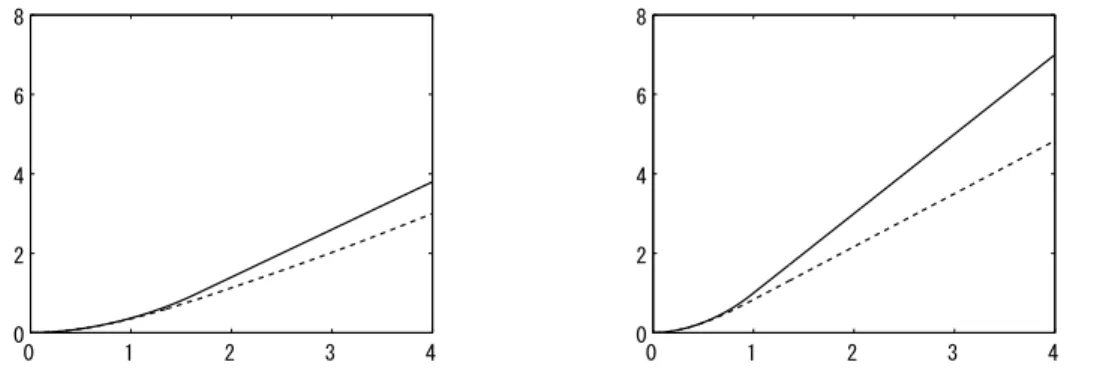
Table 2 shows how the ratio s2/s1 affects the thresholds (we fix s1 = 1). For the above parameters, case A or B in Equation (5.2) occurs according to s2 < 1.5 or s2 ≥ 1.5, respectively. In this case, an investment will be executed only when St = s2. υ2 decreases as s2 increases due to stronger incentive to invest before the Markov process moves to s1. In fact, the payoff obtained by investing at υ2 is around 1.95 for all values of s2 listed in Table 2. Figure 1 shows the value functions F1(u) and F2(u) for s2 = 1.2 and s2 = 2.0,
Table 2: s2 and threshold values υ1 and υ2 (s1 = 1)
s2 1.2 1.4 1.6 1.8 2.0
υ1 3.61 10.8 ∞ ∞ ∞
υ2 1.64 1.40 1.22 1.08 0.97
respectively. Each curve is composed of smoothly pasted 2 or 3 different functions.
0 1 2 3 4 0 2 4 6 8 0 1 2 3 4 0 2 4 6 8
Figure 1: Value functions F1(u) (dashed line) and F2(u) (solid line) for s2 = 1.2 (left panel) and s2 = 2.0 (right panel). Other parameters are the same as in Table 1
Table 3 shows thresholds when transition rates q12 and q21 of the Markov process range from 0.1 to 1.0 (from 10 years to 1 year in average). υ2 increases as q12= q21increases since the possibility of risk to stay in state s1 for longer time decreases. However, the difference is rather small for these parameters since it is almost unlikely to occur to invest in state s1. For 3-state case, we use the same parameters of µ, σ, ρ and I as in Table 1. The transition rate matrix is given by
Q = −0.5 0.5 0 0.2 −0.4 0.2 0 0.5 −0.5 . (5.15)
Table 3: Rate of regime transitions and threshold levels
q12 = q21 0.1 0.2 0.5 1.0
υ1 10.8 ∞ ∞ ∞
υ2 1.40 1.43 1.48 1.51
Since Q given in (5.15) satisfies the condition (3.7), we know υ1 ≥ υ2 ≥ υ3 in advance for
s1 < s2 < s3. Table 4 summarizes the results for s2 = 1.2, 1.4, 1.6 with s1 = 1 and s3 = 1.8 being fixed. For all values of s2, υ1 = ∞ meaning that it is never optimal to invest when
St = s1 since s1 is small compared with s3. υ2 is also infinity when s2 = 1.2 by the same reason while it becomes finite and decreases as s2increases because investment when St= s2 becomes more attractive.
Table 4: s2 and threshold values υ1, υ2 and υ3 (s1 = 1, s3 = 1.8)
s2 1.2 1.4 1.6
υ1 ∞ ∞ ∞
υ2 ∞ 9.25 2.07
υ3 1.01 1.01 1.02
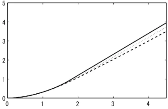
Finally, we will show an example in which all threshold values are finite. This case will occur if the difference between scale parameters are not large. Figure 2 shows the value functions for s1 = 1.00, s2 = 1.05 and s3 = 1.10 with the other parameters being the same as above. The threshold values in this case are calculated as υ1 = 4.24, υ2 = 2.32 and
υ3 = 1.75. 0 1 2 3 4 0 1 2 3 4 5
Figure 2: Value functions F1(u) (dashed line), F2(u) (dotted line) and F3(u) (solid line) Acknowledgements The author is grateful to the editors and anonymous referees for helpful comments. Especially, a comment from one of the referees lead to an extension of the original problem. He also thanks Mitsuhiko Mori for valuable discussions.
References
[1] F.-R. Chang: Stochastic Optimization in Continuous Time (Cambridge University Press, 2004).
[2] J. D´ecamps, T. Mariotti and S. Villeneuve: Irreversible investment in alternative projects. Economic Theory, 28 (2006), 425–448.
[3] A.V. Dixit and R.S. Pindyck: Investment under Uncertainty (Princeton University Press, 1994).
[4] W.H. Fleming and H.M. Soner: Controlled Markov Processes and Viscosity Solutions (Springer-Verlag, 1992).
[5] X. Guo: An explicit solution to an optimal stopping problem with regime switching.
Journal of Applied Probability, 38 (2001), 464–481.
[6] X. Guo, J. Miao and E. Morellec: Irreversible investment with regime shifts. Journal
of Economic Theory, 122 (2005), 37–59.
[7] M. Kijima: Markov Processes for Stochastic Modeling (Chapman & Hall, 1997). [8] M. Kijima: Stochastic Processes with Applications to Finance (Chapman & Hall, 2003). [9] M. Mori: Optimal investment with bivariate growth options and state dependent ca-pacity. Master thesis, Graduate School of Business Sciences, University of Tsukuba (2006).
[10] M. Ohnishi and M. Tsujimura: An impulse control of a geometric Brownian motion with quadratic costs. European Journal of Operations Research, 168 (2006), 311–321. [11] B. Oksendal: Stochastic Differential Equations, 5th ed. (Springer, 1998).
[12] E.S. Schwartz and L. Trigeorgis: Real Options and Investment under Uncertainty (MIT Press, 2004).
[13] A. Vollert: A Stochastic Control Framework for Real Option in Strategic Valuation (Birkh¨auser, 2003).
Naoki Makimoto
Graduate School of Business Sciences University of Tsukuba
3-29-1 Otsuka, Bunkyo Tokyo 112-0012, Japan