Vol. 59, No. 2, April 2016, pp. 195–217
ATTRITION GAME MODELS WITH ASYMMETRIC INFORMATION ON A NETWORK
Ryusuke Hohzaki Keiich Sunaga
National Defense Academy Japan Ministry of Defense
(Received February 23, 2015; Revised October 9, 2015)
Abstract This paper deals with two-person zero-sum (TPZS) games in which two players conflict on a network through an attrition phenomenon. The problem has a variety of applications, but we model the problem as a TPZS game with some attrition between attackers and defenders. The attackers start from a starting node and reach a destination node, expecting to keep their initial members intact. The defenders deploy their forces on arcs to intercept the attackers. If the attackers encounter defenders deployed on an arc, the attackers incur casualties proportional to the number of the deployed defenders. We discuss four games where the attackers or the defenders obtain information of their opponent. The games are two-stage games with a common payoff of the number of surviving attackers. We formulate them into linear programming problems to derive their equilibrium points and evaluate the value of the information acquisitioned in the games.
Keywords: Game theory, linear programming, attrition, network interdiction
1. Introduction
Morse and Kimball [26] first dealt with an attrition game played on networks in their well-known book Methods of Operations Research. They discussed passage interdiction against a submarine by anti-submarine warfare (ASW) airplanes in straits having shapes of rectangles or lattices. Such an inspection game originated from Dresher [13] although it was not modeled on any network, as Hohzaki [19] surveyed. Dresher, who is famous as the developer of the prisoner’s dilemma game, first discussed the inspection game to analyze arms reduction treaties, in particular with respect to the effectiveness of on-site inspections. The inspection game had a branch of research fields, smuggling games with two competi-tors, Customs and a smuggler, during the 1980s and 1990s to solve serious drug problems in the U.S. Thomas and Nisgav [36] contributed to the early development of the smug-gling game. The smugsmug-gling game is usually modeled as an ordinary multi-stage game not involving a network but some researchers consider interdiction on smuggling networks con-sisting of transportation routes of illegal drugs or other contraband, such as Mitchell and Bell [25], Caulkins, Crawford, and Reuter [10], Washburn and Wood [37] and Salmeron [32]. Washburn and Wood, in particular, applied graph theory and game theory to their network model.
We refer to the interdiction problem on a network as the network interdiction model, which includes the smuggling game mentioned above. The network interdiction model can also be applied to many other real-world problems, such as tactical air strikes, infection control in a hospital, chemical treatment of raw sewage, flood control, and maintaining infrastructure resilience against various types of attacks. There has been much research on these topics.
Ford and Fulkerson [14], and Wollmer [39] analyzed the effect of destruction of arcs on some characteristic indices of networks. McMasters and Mustin [24], and Ghare et al. [16] discussed the damage on logistics by destroying its network structure. Fulkerson and Harding [15], and Golden [18] considered how to extend the total length of the shortest path as much as possible under a limited destruction budget assuming the damage on an arc bears the increase of its length. Cappanera and Scaparra [9] discussed an optimal allocation of protective resource in shortest path networks. Wood [40] discussed a Stackelberg game on a maximum flow on a network. Bakir [6] also considered a Stackelberg game on the interdict of an unauthorized weapon insertion via sea ports or other points. Akgun et al. [2] also dealt with a Stackelberg game on an interdiction problem of multi-commodity maximum flows. Whiteman [38] and Brown et al. [8] studied military applications of network interdiction games.
Assimakopoulos [4] formulated a model of optimal interdiction of the infection network in a hospital and Salmeron et al. [33] considered a game to mitigate the damage on electric power grids attacked by terrorists. Kodialam and Lakshman [21] developed a sampling method of inspecting data packets to detect the intrusion of a computer virus or other illegal software. Church et al. [11], Scaparra and Church [34], and Desai and Sen [12] discussed defense problems of facilities.
As for network design problems to guarantee the reliability of communication, Gibbens and Kelly [17], and Ouveysi and Wirth [28] discussed flexible networks to be resilient against the deletion of arcs. Smith et al. [35] discussed fortification of a telecommunication network against malicious attacks. Alveras et al. [3] and Myung et al. [27] considered network design problems to secure the required communication flows in a mobile phone network and a telecommunication network, respectively, against the malfunction of some nodes. Regarding public transportation, Perea and Puerto [29] considered a design problem of railway networks against intentional attacks and Bell et al. [7] analyzed the vulnerability of physical road networks under threat of attack by terrorists from a game-theoretical point of view.
We generally assume the conservation of flows on networks in graph theory. However we can handle the flow to be lost or gained on the way by the concept of generalized flow. Lawler [23] and Ahuja, et al. [1] developed their theory on the generalized flow and mentioned some practical applications.
Ruckle [30, 31] developed an original ambush game, in which Blue team wishes to move across a rectangular lattice in such a way as to avoid being ambushed by Red team, who places obstacles in Blue’s paths. The interdiction game is sometimes called the infiltration
game [5] from the standpoint of the intruder.
Hohzaki and Chiba [20] first applied the interdiction model to an attrition game, in which attackers and defenders compete with each other on a network. The attackers march from a starting node to a destination node, expecting to keep their initial members intact during the march. The defenders deploy their forces on arcs to intercept the attackers. If the attackers encounter deployed defenders on an arc, the attackers incur casualties according to Lanchester’s linear law on attrition. They model the attrition game with no information as a one-shot two-person zero-sum (TPZS) game and another game with the acquisition of information about players’ opponents as a two-stage TPZS game. The payoff of both games is defined as the number of attackers arriving at the destination node. They developed linear programming formulations to derive equilibrium points of the games. In the game, the players could obtain several kinds of information and then we have a variety of situations of information acquisition. Hohzaki and Chiba dealt with just a case of them. Therefore,
we cannot say that they comprehensively evaluated the value of information. We know that different information has different effects on an equilibrium point of game even if the framework of the game is the same. In this research, we focus on the valuation of various information, which players could obtain while playing the attrition game, in an exhaustive and comprehensive manner by considering several types of information in formulating two-stage games. We have an ultimate purpose to clarify a full-spectrum relationship between the information and the equilibrium point in the research field of the attrition game although we are required to accumulate more research in the future.
In the next section, we review the one-shot game and the two-stage game of Hohzaki and Chiba [20], from which our models are branched, as a preliminary. In Section 3, we model four situations under which players obtain asymmetric information and formulate them into two-stage games and propose some methods to derive equilibrium points. In Section 4, we take some numerical examples to analyze the characteristics of optimal strategies and the effect of information involved in the games by sensitivity analyses. Finally we conclude our research with some remarks in Section 5.
2. Basic Model of the Attrition Game and its Equilibrium
We consider an attrition game, in which attackers and defenders compete with each other on an acyclic directed network and players get asymmetric information of their opponents in the conflict. Because two competitors are often called Red and Blue, we implicitly regard the attackers as Red (R) and the defenders as Blue (B). Our model originates from Hohzaki and Chiba’s study [20]. They discussed a one-shot attrition game without any information and also considered a two-stage game with information acquisition by both players. As a preliminary of our model, let us outline their results in the following section.
2.1. One-shot game and its equilibrium
Here we consider the following model of one-shot attrition game.
A1. The space is a directed network, denoted by G(N , A), consisting of a set of nodes
N and a set of directed arcs A. G(N , A) is an acyclic network, in which there is no
directed cycle. On the network, there is a direct path at the least from a specific node
s to another specific node t.
A2. There are two players, attackers and defenders. The attackers start from the start node s and attempts to arrive at the destination node t while maintaining as many members as possible. The initial number of attacking members is R0 at node s. The
defenders want to reduce the attacking forces on their way to t by deploying B0 initial
members on arcs. Let us regard the number of members as a real number.
A3. On each arc, the attackers incur some attrition, i.e. casualties, due to collision with the defenders deployed there. As a result of the collision between x attackers and y defenders on arc e, the number of surviving attackers after attrition, fe(x, y), obeys the following rule.
fe(x, y) = max{0, x − γey} (2.1)
In Equation (2.1), coefficient γe indicates the relative strength of the defenders against the attackers on the arc e and is called the exchange rate.
A4. Both players make their decision without any information of their opponents.
A5. Both players are interested in the number of surviving attackers at the final node t. The attackers desire to maximize the number, whereas the defenders want to minimize it.
Equation (2.1) in Assumption A3 is called Lanchester’s linear law in attrition theory and the coefficient γeis given as a ratio, γe = be/re, where beand reare the so-called kill rates of the defender’s power and the attacker’s power, respectively. In the linear law, the amounts of attrition on the two sides are assumed to be proportional to each other, as follows.
X0− X = γe(Y0− Y ),
where X0 and Y0 are the initial numbers of attackers and defenders, respectively, and X and
Y are the numbers of respective sides at the present time. Therefore, if each player fights
his enemy until his exhaustion, Y = 0 or X = 0, then the number of surviving attackers or defenders would be X = max{0, X0− γeY0} or Y = max { 0, Y0− 1 γe X0 } . (2.2)
Even though Assumption A2 allows the attackers to dispatch several groups of their members by some different paths separately, we consider the attacker’s strategy of marching a unified team on a path because any former strategy (splitting strategy) is dominated by some latter strategy (concentrated-flow strategy), as Hohzaki and Chiba [20] proved. Therefore, a pure strategy of the attackers is a choice of their marching path.
Let us denote all paths from node s to t by Ω and all arcs included in path ℓ ∈ Ω by
Eℓ ⊆ A. A pure strategy of the defenders is a deployment plan of their members represented
by a vector y = {ye, e ∈ A}, where ye is the number assigned on arc e. A pure strategy of the attackers is a choice of a path ℓ ∈ Ω. In the following discussion, we take a mixed strategy π ={π(ℓ), ℓ ∈ Ω} for the attackers, where π(ℓ) is the probability of taking path ℓ. Let us derive the payoff of the game. From Eqs. (2.2), the attackers taking path ℓ have the number of surviving members, max{0, R0−
∑
e∈Eℓγeye}, at the destination node t. By an attacker’s mixed strategy π and a defender’s pure strategy y, the expected number of surviving attackers, R(π, y), is given by
R(π, y) =∑ ℓ∈Ω π(ℓ) max { 0, R0− ∑ e∈Eℓ γeye } . (2.3)
Because the expected payoff is linear for π and convex for y, we already know that the game has an equilibrium point as a combination of π and y from theory on convex game. We can derive an optimal defender’s strategy y∗ by solving the minimax optimization problem of the expected payoff (2.3) and an optimal attacker’s strategy π∗ by solving the maximin optimization one.
We leave the detail of the derivation of the equilibrium to the reference [20] and we review just a theorem on the equilibrium.
Theorem 2.1 (One-shot attrition game and its equilibrium[20]). As for the equilibrium
of the one-shot attrition game, an optimal defender’s strategy y∗ is given by an optimal
optimal solution of problem (MII R). (MBI′) min y,ξ ξ s.t. ξ≥ 0, ξ≥ R0− ∑ e∈Eℓ γeye, ℓ ∈ Ω, (2.4) ∑ e∈A ye ≤ B0, ye ≥ 0, e ∈ A. (MRII) max π,ρ,λ ( R0 ∑ ℓ∈Ω ρ(ℓ)− B0λ ) (2.5) s.t. ρ(ℓ)≤ π(ℓ), ℓ ∈ Ω, γe ∑ {ℓ|e∈Eℓ} ρ(ℓ)≤ λ, e ∈ A, (2.6) ρ(ℓ)≥ 0, ℓ ∈ Ω, ∑ ℓ∈Ω π(ℓ) = 1, π(ℓ)≥ 0, ℓ ∈ Ω.
y∗ and π∗ are also dual variables corresponding to condition (2.6) and (2.4), respectively.
As seen from condition (2.4), the optimal defense strategy makes the maximal number of surviving attackers among for all paths as minimal as possible, that is, it responds better to whichever path the attackers take.
2.2. Two-stage game and its equilibrium
Here we substitute the following assumption for Assumption A4 without changing any other assumptions of the previous model.
B4. At one point in time after the attackers started marching, the defenders know the present node of the attackers and the number of remaining attackers. At the same time, the attackers obtain information of the number of defenders to be positioned thereafter. This information acquisition takes place when the attackers are at node Nℓ for their arbitrary path ℓ. The defenders deployed before the information acquisition are not available anymore after that.
In this game, we have two stages: the stage before information acquisition (Stage 1) and the stage after then (Stage 2). We denote a mixed attacker’s strategy at Stage 1 by π(ℓ), where π(ℓ) is the probability of taking path ℓ, and a mixed one at Stage 2 by πℓ(ℓ′), which is the probability of taking path ℓ′ ∈ PNℓ
t at Stage 2 after taking path ℓ at Stage 1 and reaching the node of information acquisition Nℓ. Pji is a set of all paths from node i to j. For the defender’s side, y(1) ={y(1)e , e ∈ A} is a strategy at Stage 1 and {y(2)e , e ∈ A} is a strategy at Stage 2, which is the deployment of residual attackers of B0−
∑ e∈Ay
(1)
e on arcs. Let Eℓ(1) be the arcs that path ℓ goes through at Stage 1.
Let Γ(R0, s, B0) be the one-shot game modeled in Section 2.1 and v(R0, s, B0) be the
value of the game. Thus, game Γ(R, N, B) is the one-shot game with an initial number
attackers take path ℓ ∈ Ω and the defenders use a strategy y(1) at Stage 1, the attackers
have their residual number R(ℓ, y(1))≡ max{0, R0−
∑
e∈Eℓ(1)γey (1)
e } when they start from the
information acquisition node (the IA node) Nℓ in the beginning of Stage 2. The defenders have B2(y(1))≡ B0−
∑ e∈Ay
(1)
e forces available at Stage 2. Therefore, players would fight the one-shot game Γ(R(ℓ, y(1)), Nℓ, B2(y(1))) at Stage 2 and the payoff v(R(ℓ, y(1)), Nℓ, B2(y(1)))
is born. As for the planning for Stage 1, both players decide their strategies of the path selection ℓ and the defense deployment y(1) in a rational way by estimating the result of the
game at Stage 2.
Unless the defense plan y(1) at Stage 1 is specifically given, it seems that we cannot
calculate R(ℓ, y(1)) and B
2(y(1)), and cannot apply the formulation in Section 2.1 to the
calculation of the payoff v(·). Practically it is easy to estimate the attrition of the attackers at Stage 2, w∗(ℓ, y(1)), by the equilibrium strategies of the game of Stage 2, as Hohzaki and
Chiba [20] showed. According to their theory, the expectation of attrition at Stage 2 is given by the product of the residual number of defenders, B0−
∑ e∈Ay
(1)
e , and the optimal value of the following problem, νℓ∗, just depending on IA node Nℓ. That is, νℓ∗ is an attrition rate during Stage 2 for the attackers starting from the IA node Nℓ.
(D2ℓ) νℓ∗ = min νℓ,λℓ(ℓ′) νℓ s.t. νℓ− γe ∑ ℓ′∈PtNℓ|e∈Eℓ′ λℓ(ℓ′)≥ 0, e ∈ A, ∑ ℓ′∈PtNℓ λℓ(ℓ′) = 1, λℓ(ℓ′)≥ 0, ℓ′ ∈ PtNℓ.
Furthermore the optimal variable λℓ(ℓ′) of the problem is an optimal attacker’s strategy
πℓ∗(ℓ′) at Stage 2. From the discussion so far, we have the payoff brought by an attacker’s strategy ℓ∈ Ω and a defender’s strategy y(1), as follows.
R0− ∑ e∈E(1)ℓ γey(1)e − νℓ∗ ( B0− ∑ e∈A ye(1) ) .
By applying the formulation (MI′
B) to the payoff, we have the following linear programming problem to derive an optimal defender’s strategy y∗(1) at Stage 1.
(T1) min µ(1),y(1)µ (1) s.t. µ(1) ≥ R0− ∑ e∈E(1)ℓ γey(1)e − νℓ∗ ( B0− ∑ e∈A ye(1) ) , ℓ∈ Ω, µ(1) ≥ 0, ∑ e∈A y(1)e ≤ B0, y(1)e ≥ 0, e ∈ A.
Theorem 2.2 (Equilibrium of the two-stage game [20]). We can calculate an equilibrium
νℓ∗. Using νℓ∗, solve the problem (T1) and another linear problem (V
1) given below to derive
optimal strategies y∗(1) and π∗ at Stage 1.
(V1) max π,η R0− B0 ∑ ℓ∈Ω π(ℓ)νℓ∗− B0η s.t. ∑ ℓ∈Ω π(ℓ)νℓ∗− γe ∑ ℓ∈Ω(1)e π(ℓ)≥ −η, e ∈ A(1), η ≥ 0, ∑ ℓ∈Ω π(ℓ) = 1, π(ℓ)≥ 0, ℓ ∈ Ω,
where A(1) is all arcs some path passes through at Stage 1 and Ω(1)e is a set of paths going
through arc e at Stage 1, defined by Ω(1)e ≡ {ℓ ∈ Ω|e ∈ Eℓ(1)}.
We can calculate optimal strategies at Stage 2 by applying the formulations given in Section 2.1 to the one-shot game Γ(R, i, B) knowing the current attackers’ position, say i, the number of surviving attackers, R, and the number of available defenders, B, at the beginning of Stage 2.
3. Attrition Games with Asymmetric Information
Here we consider two-stage games under various situations of acquisition of asymmetric information. As same as the two-stage model in Section 2.2, players acquire information of their opponents at the IA node Nℓ if the attackers take a path ℓ at Stage 1. Before the discussion, let us define notations, some of which might appear in previous sections.
Notations
• Ω: All paths moving from node s to t • Pi
j: All paths moving from node i to j
• Eℓ: Arcs on path ℓ
• E(1)
ℓ : Arcs that path ℓ goes through at Stage 1
• E(2)
ℓ : Arcs that path ℓ goes through at Stage 2
• E(2) Nℓ(ℓ
′): Arcs that path ℓ′ starting from IA node N
ℓ goes through at Stage 2; ≡ E (2) ℓ′
• Ω(1)
e : A set of paths going through arc e at Stage 1; ≡ {ℓ ∈ Ω|e ∈ Eℓ(1)}
• ΩP: A set of paths going through node P
• bγℓ: The minimum among the maximal exchange rates of arcs on each path ℓ′ passing through node Nℓ;≡ minℓ′∈ΩNℓ maxe∈E(2)
ℓ′
γe
• A(1): A set of arcs that any path passes by at Stage 1; ≡∪ ℓ∈ΩE
(1) ℓ
3.1. A model that the defenders have perfect information of the attackers We change Assumption A4 in Section 2.1 to the following.
C4. When the attackers reach node Nℓ on their arbitrary path ℓ at Stage 1, the defenders know the current position of the attackers Nℓ, the number of surviving attackers and the path the attackers move along since then. The attackers know nothing about the defenders but just knows that the defenders get information of them.
Let denote an attacker’s strategy and a defender’s strategy at Stage 1 by π and y(1),
re-spectively, as in Section 2.2. In the case that the attackers move on path ℓ against the defender’s plan y(1) at Stage 1, the defenders know the attackers’ path ℓ′ ∈ ΩNℓ at Stage 2
so that they puts all their forces of B0−
∑ e∈Ay
(1)
e on hand on the most effective arc with the maximum rate of maxe∈E(2)
ℓ′
γe. Noticing that, the attackers should choose a path with the arc having the minimum one of the maximum rates. In the result, at Stage 2, a combat deterministically occurs on the arc with the rate bγℓ ≡ minℓ′∈ΩNℓmaxe∈E(2)
ℓ′
γe between the attackers and the defenders. We refer to bγℓ as the minimax exchange rate for the path ℓ. The residual number of attackers is estimated as follows.
R(ℓ, y(1)) = max 0, R0− ∑ e∈Eℓ(1) γey(1)e − bγℓ ( B0− ∑ e∈A ye(1) ) . (3.1)
Therefore, the expected payoff is given by R(π, y(1)) =∑
ℓ∈Ωπ(ℓ)R(ℓ, y
(1)) at Stage 1. We
optimize the expected payoff to derive players’ optimal strategies. Minimax optimization: From the transformation
min
y(1) maxπ R(π, y
(1)) = min
y(1) maxℓ∈Ω R(ℓ, y
(1)) = min µ s.t. R(ℓ, y(1))≤ µ, ℓ ∈ Ω,
we have the final formulation for the minimax optimization, as follows.
(DPB) min y(1),µµ s.t. µ≥ R0− ∑ e∈Eℓ(1) γey(1)e − bγℓ ( B0− ∑ e∈A ye(1) ) , ℓ∈ Ω, (3.2) µ≥ 0, (3.3) ∑ e∈A ye(1)≤ B0, ye(1) ≥ 0, e ∈ A.
We obtain an optimal defender’s strategy y∗(1) at Stage 1 by solving the problem (DPB). Anyways, an optimal defending strategy at Stage 2 is to deploy B0 −
∑ e∈Ay
∗(1)
e available
defenders on the arc e∗ of e∗ = arg maxe∈E(2) ℓ′
γeafter the defenders know the attacker’s path
ℓ′ at the beginning of Stage 2.
Maximin optimization: The problem of miny(1) ∑
ℓ∈Ωπ(ℓ)R(ℓ, y
(1)) is formulated into the
followings. min y(1),µ ∑ ℓ∈Ω π(ℓ)µℓ s.t. µℓ ≥ 0, ℓ ∈ Ω, µℓ ≥ R0− ∑ e∈E(1)ℓ γeye(1)− bγℓ ( B0− ∑ e∈A ye(1) ) , ℓ∈ Ω, (3.4) ∑ e∈A y(1)e ≤ B0, (3.5) y(1)e ≥ 0, e ∈ A.
Setting dual variables ξℓ and λ corresponding to Eqs. (3.4) and (3.5), respectively, we generate the following problem dual to the above problem.
max ξ,λ ∑ ℓ∈Ω ξℓ(R0− bγℓB0)− λB0 s.t. ξℓ ≤ π(ℓ), ℓ ∈ Ω, − ∑ ℓ∈Ω(1)e ξℓ(bγℓ− γe)− ∑ ℓ∈Ω\Ω(1)e ξℓbγℓ− λ ≤ 0, e ∈ A, ξℓ ≥ 0, ℓ ∈ Ω, λ≥ 0.
We further maximize the maximum value obtained above with respect to π to obtain the maximin value of the game.
(DPR) max π,ξ,λ ∑ ℓ∈Ω ξℓ(R0− bγℓB0)− λB0 s.t. ξℓ ≤ π(ℓ), ℓ ∈ Ω, (3.6) 0≤ ξℓ, ℓ∈ Ω, λ + ∑ ℓ∈Ω(1)e ξℓ(bγℓ− γe) + ∑ ℓ∈Ω\Ω(1)e ξℓbγℓ ≥ 0, e ∈ A, (3.7) λ ≥ 0, ∑ ℓ∈Ω π(ℓ) = 1. (3.8)
The problem gives us an optimal attacker’s strategy π∗ at Stage 1. At Stage 2, the attackers have to choose ℓ∗ = arg minℓ′∈ΩNℓmaxe∈E(2)
ℓ′
γe if they take path ℓ at Stage 1.
We can prove that the problems (DPB) and (DPR) have the same optimal value and there exists an equilibrium point as a combination of an attacker’s mixed strategy and a defender’s pure strategy. Setting dual variables σℓ, ye and µ corresponding to conditions (3.6), (3.7) and (3.8), respectively, we generate a dual problem of (DPR), as follows.
min y,σ,µµ s.t. σℓ ≥ R0− ∑ e∈Eℓ(1) γeye− bγℓ ( B0− ∑ e∈A ye ) , ℓ∈ Ω, (3.9) µ≥ σℓ, ℓ∈ Ω, (3.10) σℓ ≥ 0, ℓ ∈ Ω, (3.11) ∑ e∈A ye ≤ B0, ye ≥ 0, e ∈ A.
We can make condition (3.2) from inequalities (3.9) and (3.10), and condition (3.3) from (3.10) and (3.11). Conversely, we can also easily generate feasible variables σℓ satisfying conditions (3.9), (3.10) and (3.11) from (3.2) and (3.3). We have confirmed that the above dual problem is equivalent to (DPB).
3.2. A model that the defenders have imperfect information of the attackers Let us consider the model with the replacement of Assumption (A4) with the followings.
D4. The defenders know the current position of the attackers, Nℓ, and the number of surviving attackers, R, when the attackers reach node Nℓ on their arbitrary path ℓ. On the other hand, the attackers never acquisition any information of the defenders but notices that the defenders know Nℓ and R.
In the model, the defenders can change their defense plan using the information about the attackers at Stage 2. The attackers can also choose their path among all paths PNℓ
t leading
from node Nℓ to t after noticing the defender’s acquisition of the information.
If the attackers knew the residual defenders’ number B, the game at Stage 2 becomes Γ(R, Nℓ, B) in Section 2.1 and both players expect the payoff v(R, Nℓ, B) because the number
R and the node Nℓ are already common knowledge. From the discussion in Section 2.2, we
see that the attrition on the attacker’s side at Stage 2 is given by the product of the optimal value νℓ∗ of problem (D2ℓ) and the defender’s resource B = B0−
∑ ey
(1) e .
In the case of the attacker’s path selection ℓ and the defender’s deployment y(1) at Stage
1, R = max{0, R0−
∑
e∈E(1)ℓ γey (1)
e } attackers would survive during Stage 1 but additional
attrition occurs to the attackers by playing the game Γ(R, Nℓ, B) during Stage 2. Therefore, we have the following payoff by the strategies ℓ and y(1) at Stage 1.
R(ℓ, y(1)) = max 0, R0− ∑ e∈Eℓ(1) γey(1)e − νℓ∗ ( B0− ∑ e∈A ye(1) ) . (3.12)
Finally, we can see that the game of Stage 1 is the one-shot game with the expected payoff ∑
ℓ∈Ωπ(1)(ℓ)R(ℓ, y(1)) for an attacker’s mixed strategy π(1) and a defender’s strategy y(1). The equilibrium of the game is easily derived in the same way as we do for the two-stage game in Section 2.2. That is, we have an optimal defender’s strategy y∗(1) by solving problem (T1) and an optimal attacker’s strategy π∗(1) by (V
1). From the discussion so far,
the attackers do not need the residual defenders’ number B to estimate y∗(1) certainly and then the equilibrium of the game becomes the same as one of the two-stage game in Section 2.2.
An optimal defender’s strategy y∗(2) at Stage 2 is derived from the following problem (S2
ℓ) by applying the obtained values y∗(1). An optimal strategy of the attackers after taking path ℓ at Stage 1 is given by λ∗ℓ(ℓ′) of problem (D2
ℓ). (Sℓ2) max µ(2),y(2)µ (2) s.t. µ(2) ≤ ∑ e∈E(2) ℓ′ γeye(2), ℓ′ ∈ ΩNℓ, (3.13) ∑ e∈A y(2)e ≤ B0 − ∑ e∈A ye∗(1), (3.14) y(2)e ≥ 0, e ∈ A.
3.3. A model that the attackers have perfect information of the defenders Here we consider the game with the replacement of Assumption A4 with the following assumption.
E4. When the attackers reach node Nℓon their arbitrary path ℓ, they know the deployment plan of the defenders in the future. The defenders notice the information acquisition by the attackers.
Under this situation, the defenders can make a decision on their defense deployment at the beginning of Stage 2 but the attackers know the decision. Hence the defenders do not need the decision making at that time and they may make their plan once at the beginning of Stage 1 while being aware well of the leakage of the plan to the attackers at Stage 2.
Because the attackers taking path ℓ know any defense plan y at the beginning of Stage 2, they choose the path ℓ∗(2)(y) = arg minℓ′∈ΩNℓ
∑
e∈ENℓ(2)(ℓ′)γeye at Stage 2. At the end of
Stage 1, the attackers have max{0, R0 −
∑
e∈Eℓ(1)γeye} survivors. In the case of players’ strategies ℓ and y at Stage 1, the final number of surviving attackers is
R(ℓ, y) = max 0, R0− ∑ e∈Eℓ(1) γeye− min ℓ′∈ΩNℓ ∑ e∈ENℓ(2)(ℓ′) γeye . (3.15)
Therefore, we would obtain an equilibrium point at Stage 1 by solving the one-shot game with the expected payoff R(π, y) =∑ℓπ(ℓ)R(ℓ, y) by a mixed attacker’s strategy π.
Minimax optimization: From a transformation
min
y maxπ R(π, y) = miny maxℓ∈Ω R(ℓ, y) = miny µ s.t. R(ℓ, y)≤ µ, ℓ ∈ Ω,
we have a linear programming problem for the minimax optimization. Its optimal variable y∗ gives us an optimal defender’s strategy. Optimal variable ηℓ gives minℓ′∈ΩNℓ
∑
e∈ENℓ(2)(ℓ′)γeye
in the problem, as seen from Equation (3.15).
(APB) min y,µ,ηµ (3.16) s.t. µ≥ R0− ∑ e∈E(1) ℓ γeye− ηℓ, ℓ ∈ Ω, (3.17) µ≥ 0, ηℓ ≤ ∑ e∈E(2) Nℓ(ℓ′) γeye, ℓ′ ∈ ΩNℓ, ℓ∈ Ω, (3.18) ∑ e∈A ye ≤ B0, ye ≥ 0, e ∈ A.
formulated into the followings. min y,ν,η ∑ ℓ∈Ω π(ℓ)νℓ s.t. νℓ ≥ 0, ℓ ∈ Ω, νℓ ≥ R0 − ∑ e∈Eℓ(1) γeye− ηℓ, ℓ∈ Ω, (3.19) ηℓ ≤ ∑ e∈E(2)Nℓ(ℓ′) γeye, ℓ′ ∈ ΩNℓ, ℓ ∈ Ω, (3.20) ∑ e∈A ye ≤ B0, (3.21) ye ≥ 0, e ∈ A.
Set variables ρ(ℓ), ξℓ(ℓ′) and λ corresponding to conditions (3.19), (3.20) and (3.21), respec-tively, and make a dual problem, then we have the followings.
max λ,ρ,ξR0 ∑ ℓ∈Ω ρ(ℓ)− B0λ, s.t. −λ + γe ∑ ℓ∈Ω(1)e ρ(ℓ) + ∑ {(ℓ,ℓ′)|e∈E(2) Nℓ(ℓ′),ℓ′∈ΩNℓ,ℓ∈Ω} ξℓ(ℓ′) ≤ 0, e ∈ A, ρ(ℓ)≤ π(ℓ), ℓ ∈ Ω, ρ(ℓ)− ∑ ℓ′∈ΩNℓ ξℓ(ℓ′) = 0, ℓ ∈ Ω, λ≥ 0, ρ(ℓ)≥ 0, ℓ ∈ Ω, ξℓ(ℓ′)≥ 0, ℓ′ ∈ ΩNℓ, ℓ∈ Ω.
Furthermore we maximize the above with respect to π to obtain a final formulation for the maximin value and an optimal path selection π∗.
(APR) max π,λ,ρ,ξR0 ∑ ℓ∈Ω ρ(ℓ)− B0λ s.t. γe ∑ ℓ∈Ω(1)e ρ(ℓ) + ∑ {(ℓ,ℓ′)|e∈E(2) Nℓ(ℓ′),ℓ′∈ΩNℓ,ℓ∈Ω} ξℓ(ℓ′) ≤ λ, e ∈ A, (3.22) 0≤ ρ(ℓ) ≤ π(ℓ), ℓ ∈ Ω, ρ(ℓ) = ∑ ℓ′∈ΩNℓ ξℓ(ℓ′), ℓ∈ Ω, (3.23) ξℓ(ℓ′)≥ 0, ℓ′ ∈ ΩNℓ, ℓ∈ Ω, (3.24) ∑ ℓ∈Ω π(ℓ) = 1. (3.25)
The attackers should optimally choose a path ℓ∗(2)(y) at Stage 2 by knowing the defense plan y, of course.
Here we notice that problem (APB) looks like (MI ′
B) for the one-shot game in Section 2.1. Practically, from conditions (3.18) and (3.17), we have the following inequality for any path ℓ′ going through node Nℓ on ℓ∈ Ω.
µ≥ R0− ∑ e∈E(1) ℓ γeye− ∑ e∈E(2) Nℓ(ℓ′) γeye. Consequently, we have µ≥ R0− ∑
e∈Eℓγeye for any path ℓ∈ Ω all through Stage 1 and 2, which is the same as the condition (2.4), and have derived the problem (MI′
B). Conversely, we can easily introduce intermediate variables ηℓ satisfying condition (3.18) into (MI
′ B) and generate the problem (APB). We complete proving the equivalence of the two problems. Reviewing that an optimal solution y∗ of the problem (MI′
B) makes the maximum number
of surviving attackers among their all paths minimum, we realize that the defender’s de-ployment y∗ has the same effect on any attacker’s path even though it is changed at the IA node.
From the discussion so far, an optimal attacker’s strategy at Stage 1, an optimal de-fender’s strategy and the game value are the same as those of the one-shot game explained in Section 2.1. This means that the information the attackers get is of no use and comes from the property that the equilibrium does not change even though one player declares his optimal strategy and the other player knows before playing the game.
3.4. A model that the attackers have imperfect information of the defenders First let us replace Assumption A4 with the following.
F4. When the attackers reach node Nℓ on their arbitrary path ℓ, they know the number of defenders available afterwards. The defenders notice the information acquisition by the attackers but cannot get any information of the attackers.
In the previous section, we see that the game is essentially equivalent to the one-shot game with no information even if the attackers have perfect information about the defenders. The reasoning leads us a conjecture: this model with imperfect information of the defenders is also the same. Let us validate the conjecture by a rigorous formulation of this model.
At Stage 2, the attackers know just the number of residual defenders but do not know the deployment positions of them. So the defenders do not need to make two plans for Stage 1 and 2 but make a plan y once for all stages. We assume that the attackers choose two strategies π ={π(ℓ), ℓ ∈ Ω} and πℓ ={πℓ(ℓ′), ℓ′ ∈ ΩNℓ, ℓ ∈ Ω} at Stage 1 and 2, respectively, without utilizing the information the attackers get.
The attrition of the attackers is expected to be ∑ℓ′∈Ω
Nℓπℓ(ℓ
′)∑ e∈E(2)
ℓ′
γeye during Stage 2 when the attackers start from node Nℓfor the selected path ℓ at Stage 1. For an attacker’s strategy π and a defender’s one y, we have the expected payoff
R(π, y) =∑ ℓ∈Ω π(ℓ) max 0, R0− ∑ e∈E(1)ℓ γeye− ∑ ℓ′∈ΩNℓ πℓ(ℓ′) ∑ e∈E(2) ℓ′ γeye . (3.26) Noting ∑ℓ′∈Ω Nℓ πℓ(ℓ ′) = 1 and ∑
ℓ∈Ωπ(ℓ) = 1, we can transform the minimax optimization
of the payoff R(π, y) into
min y maxπ,πℓ R(π, y) = min y maxℓ∈Ω max 0, R0− ∑ e∈Eℓ(1) γeye− min ℓ′∈ΩNℓ ∑ e∈E(2) ℓ′ γeye .
Therefore, we have a final formulation for the minimax optimization by introducing variables ηℓ and µ, as follows. (AIB) min y,µ,ηµ s.t. µ≥ R0− ∑ e∈E(1)ℓ γeye− ηℓ, ℓ∈ Ω, (3.27) µ≥ 0, ηℓ ≤ ∑ e∈ENℓ(2)(ℓ′) γeye, ℓ′ ∈ ΩNℓ, ℓ∈ Ω, ∑ e∈A ye≤ B0, ye≥ 0, e ∈ A.
The problem is the same as problem (APB) in Section 3.3.
We carry out the maximin optimization of the payoff (3.26), as follows. First, its mini-mization is formulated into
min y,η ∑ ℓ∈Ω π(ℓ)ηℓ s.t. ηℓ ≥ R0− ∑ e∈E(1) ℓ γeye− ∑ ℓ′∈ΩNℓ πℓ(ℓ′) ∑ e∈E(2) ℓ′ γeye, ℓ∈ Ω, (3.28) ηℓ ≥ 0, ℓ ∈ Ω, ∑ e∈A ye≤ B0, (3.29) ye≥ 0, e ∈ A.
By dual variables ρ(ℓ) and λ corresponding to conditions (3.28) and (3.29), respectively, we make a dual problem, which is furthermore maximized with respect to π and πℓ to formulate a linear programming problem for the maximin value, as follows.
(AIR) max π,{πℓ},ρ,λ R0 ∑ ℓ∈Ω ρ(ℓ)− B0λ s.t. γe ∑ ℓ∈Ω(1)e ρ(ℓ) + ∑ {(ℓ,ℓ′)|e∈E(2) ℓ′ ,ℓ′∈ΩNℓ,ℓ∈Ω} ρ(ℓ)πℓ(ℓ′) ≤ λ, e ∈ A, (3.30) ρ(ℓ)≤ π(ℓ), ℓ ∈ Ω, ρ(ℓ)≥ 0, ℓ ∈ Ω, λ≥ 0, ∑ ℓ∈Ω π(ℓ) = 1, π(ℓ)≥ 0, ℓ ∈ Ω, ∑ ℓ′∈PtNℓ πℓ(ℓ′) = 1, ℓ ∈ Ω, (3.31) πℓ(ℓ′)≥ 0, ℓ′ ∈ PtNℓ, ℓ∈ Ω. (3.32)
Let us check the equivalence of problems (AIR) and (APR) in Section 3.3. If we introduce variable ξℓ(ℓ′)≡ ρ(ℓ)πℓ(ℓ′) into (AIR), the variable is nonnegative. We also have conditions ∑
ℓ′∈ΩNℓξℓ(ℓ′) = ρ(ℓ) and then (3.22) from Equation (3.31) to derive the problem (APR). We can confirm the inverse derivation as follows. First, let us review that inequality (3.23) is exchangeable with equality. In the case of ρ(ℓ) ̸= 0, conditions (3.30), (3.31) and (3.32) hold by the introduction of variable πℓ(ℓ′) ≡ ξℓ(ℓ′)/ρ(ℓ) into (APR). In the case of
ρ(ℓ) = 0, we must have ξℓ(ℓ′) = 0 (ℓ′ ∈ ΩNℓ) from (3.23) and therefore the path ℓ and arbitrary ℓ′ ∈ ΩNℓ do not affect an optimal value of the problem (APR) at all. For the ℓ of ρ(ℓ) = 0, we have equality (3.31) because any πℓ(ℓ′)(ℓ′ ∈ ΩNℓ) is allowable in condition (3.30). We complete the derivation of the problem (AIR).
The above confirmation of the equivalence of this model and the one-shot game model, discussed in Section 3.3 and 2.1, is carried out based on the assumption that the attacker’s information on the number of available defenders is useless to the attackers. We have to explain the validity of the assumption. As seen from Equation (3.27), an optimal defender’s strategy y∗ guarantees that the number of residual attackers is µ∗ at most for any attacking path. Therefore, when the attackers choose a path ℓ′ ∈ ΩNℓ at node Nℓ after taking path
ℓ during Stage 1, they just estimates their survived number as µ∗ at most for any path ℓ′
even if they can know y∗ or the number of available defenders B = B0−
∑
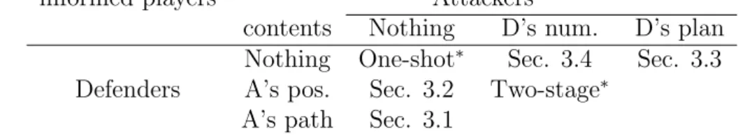
e∈Ay∗e. Thus the information of the number B cannot increase the number of surviving attackers at all. 3.5. Descriptive summary of theoretical results and valuation of information We have finished our discussion about each model in Section 3.1–3.4 from a theoretical viewpoint of formulation. For the sake of reader’s comprehensibility, however, we sum up the results of four models from a descriptive point of view. Table 1 shows the category of four models based on the contents of acquired information: attacker’s current position (A’s pos.), attacker’s future path (A’s path), the number of residual defenders (D’s num.) and defender’s deployment plan (D’s plan). The section numbers in which these models are discussed are also posted in the table.
Table 1: Category of four models based on the contents of acquired information
informed players Attackers
contents Nothing D’s num. D’s plan
Nothing One-shot∗ Sec. 3.4 Sec. 3.3
Defenders A’s pos. Sec. 3.2 Two-stage∗
A’s path Sec. 3.1
*) models developed by Hohzaki and Chiba [20]
(1) In the model that the attackers know the number of defenders available for Stage 2 (Section 3.4) and the model that the attackers know the deployment plan of the defenders at Stage 2 (Section 3.3), the defenders take a deployment plan to secure the game value against any attacker’s path and then the attacker’s acquisition of the defender’s information does not work at all to increase the number of surviving attackers. That is why their models have the same value as the one-shot game with no information on neither side of the attacker and the defender, explained in Section 2.1. We name these models Model 1 and denote its value by G1.
(2) In the model that the defenders know the position of the attackers at the beginning of Stage 2 (Section 3.2), the attackers can certainly estimate an optimal defender’s plan of Stage 1 and then the model has the same value as the two-stage game model with
some information on both sides, explained in Section 2.2. We name the model Model 2 and denote its value by G2.
(3) In the model that the defenders know the number of surviving attackers, and the current position and the future path ℓ of the attackers (Section 3.1), the defenders know the attrition rate of the attackers, bγℓ, at Stage 2 and make an optimal defense plan to intercept the attacker. We name the model Model 3 and denote its value by G3.
Considering the contents of information acquired in each model, we see a relation of G1 ≥
G2 ≥ G3 on the game value.
From the analysis above, we can say the followings on the value of information. Any information about the defenders has no value for the attackers. Because the value of Model 1 is the same as the one-shot game with no acquisition of information, a difference G12 =
G1−G2gives us the value of the information about the attackers’ position and G13 = G1−G3
the value of the information about the attacker’s path. However we must note that the information value is the reduced value under the criterion of the final number of surviving attackers, which is the payoff for every game model.
4. Numerical Examples
We have considered so far four models of the attrition game and derived an equilibrium point for each model. Consequently, as shown in Section 3.5, two models are reduced to the one-shot game model with no information (Model 1) and another model is equivalent to the two-stage game model with some information about both players (Model 2). The last model (Model 3), however, has a unique formulation. We also clarified the relation between the values of these game models. Here we analyze the characteristics of optimal strategies of players and the value in these models. We give more detailed analysis on Model 3 but an outline for Model 1 and 2 because the latter two models are essentially the same as the already-studied model by Hohzaki and Chiba [20].
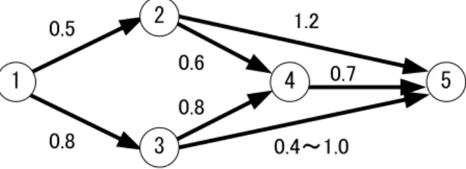
Let us consider an attrition game on a network G(N , A) with five nodes N ={1, · · · , 5} and seven directed arcs A, as illustrated by Figure 1. A number beside each arc e is the exchange rate γe. We change only γ35 from 0.4 through 1.0 to investigate the change of
equilibrium of each model. The total number R0 = 12 of attackers are going to move from
node s = 1 to t = 5. The defenders have their resource B0 = 12 for the defense on arcs. The
attackers have four options of paths ℓ = 1,· · · , 4. Path 1 moves through nodes {1, 2, 5}. Paths 2, 3 and 4 go through nodes{1, 2, 4, 5}, {1, 3, 4, 5} and {1, 3, 5}, respectively. The IA nodes are N1 = N2 = 2 for paths 1 and 2, and N3 = N4 = 3 for paths 3 and 4. Figure 2
5 1 3 2 0.5 0.8 1.2 0.6 0.8 0.4~1.0 0.7 4
Figure 1: An attrition network
shows the change of the values G1, G2 and G3 for Model 1, 2 and 3, respectively. Let us
0.0 2.0 4.0 6.0 8.0 10.0 0.4 0.5 0.6 0.7 0.8 0.9 1 γ35 V al ue o f th e ga m e G1 G2 G3
Figure 2: Value of the game
Model 1:
(1) The defenders should concentrate their defensive resource into two arcs (1, 2) and (1, 3) by the deployment of y12∗ = 7.38 and y∗13 = 4.62 at Stage 1 without dispersing them during two stages. The attackers have their residual number G1 = 8.31 at last
whichever path they take against the defense plan. Therefore, any information about the defenders is useless for the attackers to increase the payoff. The deployment remains optimal irrespective of γ35 and the game value is always G1 = 8.31.
Model 2: Table 2 shows equilibria for varying γ35 in terms of an optimal defense y∗(1)
and an optimal path selection π∗ at Stage 1, the value G2 and the attrition rate νℓ∗ which is calculated from problem (D2
ℓ). Because paths 1 and 2 have the same IA node 2 and go through the same arc (1, 2) at Stage 1, it must be that ν1∗ = ν2∗ and π∗(1) = π∗(2). Similarly, we have ν3∗ = ν4∗ and π∗(3) = π∗(4).
Table 2: Change of equilibrium points of Model 2 for γ35 = 0.4∼ 1.0
γ35 y∗(1)12 y ∗(1) 13 π∗(1) = π∗(2) π∗(3) = π∗(4) G2 ν1∗ = ν2∗ ν3∗ = ν4∗ 0.4 0 2.158 0.273 0.227 7.649 0.442 0.267 0.5 0 1.726 0.263 0.237 7.458 0.442 0.308 0.6 0 1.324 0.254 0.246 7.280 0.442 0.343 0.7 0 0.950 0.246 0.254 7.115 0.442 0.373 0.8 0 0.600 0.238 0.262 6.960 0.442 0.400 0.9 0 0.272 0.230 0.270 6.815 0.442 0.424 1 0.056 0 0.443 0.057 6.692 0.442 0.444
(1) The attrition rate ν1∗ = ν2∗ remains constant 0.442 at Stage 2 because the exchange rates of arcs on paths ℓ = 1, 2 are fixed. The rate ν3∗ = ν4∗ of paths 3 and 4 is getting larger from ν3∗ = ν4∗ = 0.267 in the case of γ35 = 0.4 as γ35 increases. Even in the
case of γ35 = 0.9, ν3∗ = ν4∗ becomes 0.424, which is smaller than ν1∗. To compensate
the lower attrition rate for paths 3 and 4 at Stage 2, the defenders put a small number of members just on arc (1, 3) at Stage 1 during γ35 = 0.4 ∼ 0.9. For example, They
have the deployment y∗(1)13 = 2.158 for γ35 = 0.4 and y13∗(1) = 0.272 for γ35 = 0.9. In the
case of γ35 = 1.0, however, ν3∗ = ν4∗ = 0.444 is larger than ν1∗ and the defenders deploy
y∗(1)12 = 0.056 on arc (1, 2), which has its exchange rate γ12 = 0.5 larger than the rate
At Stage 2, the defenders focus their deployment on arcs with larger exchange rates, through which the attackers possibly pass, after the observation of the attacker’s posi-tion, node 2 or 3. In the case of γ35= 0.4, for example, the defenders put y∗(2)25 = 3.626
and y45∗(2) = 6.216 on arcs (2, 5) and (4, 5) to intercept the node 2-passing attackers or y34∗(2) = 3.281 and y35∗(2) = 6.561 on arcs (3, 4) and (3, 5) against the node 3-passing attackers.
(2) Optimal path selection probabilities of the attackers at Stage 2 are 0.368 and 0.632 for paths 1 and 2, respectively, after node 2, and 0.368 and 0.632 for paths 3 and 4, respectively, after node 3. After passing through node 3, the attackers are less likely to take path 4 for increasing γ35.
At Stage 1, the attackers adjust π∗(1) = π∗(2) and π∗(3) = π∗(4) for paths 1,· · · , 4 in an adaptive manner, taking account of attrition rates ν1∗ = ν2∗ and ν3∗ = ν4∗ at Stage 2. As seen in (1) above, ν1∗ > ν3∗ holds for γ35= 0.1∼ 0.9 and the deployment y13∗(1) on arc
(1, 3) decreases because of increasing γ35. The tendency makes π∗(3) and π∗(4) larger.
In the case of γ35 = 1.0, an inverse relation ν1∗ < ν3∗ and γ12 < γ13 makes π∗(1) and
π∗(2) rather larger for paths 1 and 2, compared to π∗(3) and π∗(4) for paths 3 and 4. (3) As explained above, as γ35increases, the attrition rates ν3∗ and ν4∗ at Stage 2 is getting
larger and then the game value G2 decreases.
Model 3: By the same reason we have in Model 2, equalities π∗(1) = π∗(2) and π∗(3) =
π∗(4) hold. Table 3 shows optimal strategies y13∗ , π∗(1) = π∗(2) and π∗(3) = π∗(4) at Stage 1, G3, and attrition rates bγ1 =bγ2 and bγ3 =bγ4 at Stage 2.
Table 3: Change of equilibrium points of Model 3 for γ35 = 0.4∼ 1.0
γ35 y13∗ π∗(1) = π∗(2) π∗(3) = π∗(4) G3 bγ1 =bγ2 bγ3 =bγ4 0.4 3.273 0.182 0.318 5.89 0.7 0.4 0.5 2.400 0.150 0.350 5.28 0.7 0.5 0.6 1.333 0.111 0.389 4.53 0.7 0.6 0.7 0 0.231 0.269 3.60 0.7 0.7 0.8 0 0.5 0 3.60 0.7 0.8 0.9 0 0.5 0 3.60 0.7 0.8 1 0 0.5 0 3.60 0.7 0.8
(1) Starting from the IA node 2, the attackers choose path 2 and a conflict occurs on arc (4, 5) with the attrition rate bγℓ = 0.7 between the attackers and the defenders. From the other IA node 3, the attackers go along path 4 and fights the defenders on arc (3, 5) with the attrition rate bγ3 =bγ4 = γ35in the case of γ35 < 0.8 but they choose path 3 and
fight on arc (3, 4) with the attrition rate bγ3 = bγ4 = 0.8 in the case of γ35 > 0.8. Thus
we can see the followings. In the case of γ35 < 0.7, the attrition rate for the attackers
starting from node 3 is less than the attrition rate 0.7 for the attackers from node 2. To compensate the lower attrition rate for paths 3 and 4, the defenders deploy a small number of defenders y13∗(1)on arc (1, 3), which has the exchange rate γ13= 0.8 larger than
0.7. In the case of γ35 ≥ 0.7, the attrition rate for the attackers from node 3 becomes
larger than that from node 2. But the defenders do not defend arc (1, 2) to compensate the lower attrition rate for paths 1 and 2 because its exchange rate γ12= 0.5 is smaller
than 0.7. The defenders make a decision of no deployment at Stage 1 but a focused deployment of all members on Stage 2.
(2) Figure 3 shows the path selection probabilities π∗ at Stage 1 with respect to γ35. As
and then π∗(3) = π∗(4) is larger than π∗(1) = π∗(2) although the defenders deploy y13∗(1) members on arc (1, 3) to balance between the attrition on the attackers passing through IA nodes 2 and 3.
As γ35 is getting larger from 0.4 through 0.6, the defenders need a smaller y13∗ for the
balance because of the increasing efficiency of attrition on arc (3, 5). Considering the smaller deployment, the attackers take paths 3 or 4 with larger probability. At the point of γ35 = 0.7, bγℓ is 0.7 for every path ℓ and then the path selection probability approximately becomes equal for every path. When γ35 increases more, bγℓ for paths 1 and 2 at Stage 2 and γe of arcs on these paths at Stage 1 are less than for paths 3 and 4, and then the attackers use only the former paths with probabilities π∗(1) = π∗(2) = 0.5. Now we have reasonably validated the change of π∗ that π∗(1) and π∗(2) gradually decrease first as γ35 increases from 0.4 but suddenly lifts up to a maximum 0.5 for
γ35 > 0.7.
(3) Let us check the change of the game value G3 in Figure 2 and Table 3. As seen in (2)
above, the attackers choose paths 3 and 4 with larger probabilities than π∗(1) = π∗(2) in the case of γ35 ≤ 0.7. After the IA node 3, they take path 4 and go through arc (3, 5).
That is why G3 is decreasing for γ35. In the other case of γ35 > 0.7, the attackers do not
use paths 3 and 4, and do not pass through arc (3, 5). γ35 has no effect on G3 anymore.
Lastly, let us evaluate the value of information in three models. As we explained in Section 3.5, the game values G1, G2 and G3 have a relation G1 ≥ G2 ≥ G3. We can easily examine
the validity of the relation by Figure 2. Figure 4 illustrates the values of information about the attacker’s position (G12) and the attacker’s future path (G13). Our analysis on the
change of the values G1, G2, G3 also gives us a rational explanation about the change of
G12 and G13 in Figure 4. In general, the value G13 is quite large compared to G12 and both
values increase for γ35. But when γ35 becomes larger than 0.7, G13 stops increasing because
rational attacker’s paths do not go through arc (3, 5).
0.0 0.1 0.2 0.3 0.4 0.5 0.6 0.7 0.8 0.9 1.0 0.4 0.5 0.6 0.7 0.8 0.9 1 γ35 P at h se le ct io n pr o ba bi lit y π*(1)=π*(2) π*(3)=π*(4)
Figure 3: Path selection probability
0.0 1.0 2.0 3.0 4.0 5.0 0.4 0.5 0.6 0.7 0.8 0.9 1 γ35 V al ue o f in fo rm at io n G12 G13
Figure 4: Value of information
By numerical examples above, we analyzed the effect of the exchange rate γ35of arc (3, 5)
on the optimal strategy and the information value in Model 1, 2 and 3. The characteristics we found there deeply depend on the information acquisition of each model. Even in the same model, we cannot easily extract common characteristics which are always valid for all cases but we need concrete reasoning on a case-by-case basis from several points of view: Do the attackers go through relevant arcs? Do the defenders deploy any force on relevant arcs? If so, what is the attrition efficiency estimated on paths and through stages in consideration of the relative magnitude of the exchange rates of the arcs, the network configuration and
other parameters. We can do it in a numerical way, of course, by our proposed methods. We can utilize our methods for the design of networks with attrition, the setting of information acquisition nodes, the selection of arcs and the increase of their exchange rates to improve the defensive strength against the attackers from the defender’s point of view and other analyses.
5. Conclusions
In this paper, we consider the rational decision making of the attackers and the defenders in several attrition games on a network, where players obtain asymmetric information of their opponents. The game models are rather simpler than realistic problems and they include a few types of information: the number of surviving attackers, the present position and the marching route as the attacker’s information, and the number of residual defenders and the deployment plan of their forces as the defender’s information. We deal with four models to formulate them into linear programming problems for their equilibrium points. If the information brings some benefits to players, its value might be embedded in the formulations, implicitly in many cases. On the other hand, if a player can anticipate the information from a rational estimation on other players’ optimal strategies, the information is useless to the player. We handle both cases in this paper.
The anticipation by the equilibrium points has different meanings depending on whether the optimal strategy is given by a pure strategy or a mixed strategy. If the player has the former anticipation, the player could substitute the anticipation for authentic information because the anticipation is certain. In the case of the latter anticipation by a mixed strat-egy, the anticipation is probabilistic and uncertain, and the information about the actual behavior of a player has some values for the other player to know.
As in the previous research by Hohzaki and Chiba [20], we could derive the equilibrium of every attrition game ruled by Lanchester’s linear law as a combination of an attacker’s mixed strategy and a defender’s pure strategy. Therefore we can say that the information of the attackers is generally more valuable than one of the defenders. Practically, we de-rived a formulation involving the parameter bγℓ of indicating the value of information about the attacker’s future path ℓ in Model 3. By an example of Model 3, we also numerically showed that by making use of the information, the defenders can considerably decrease the expected number of surviving attackers compared to a corresponding one-shot game with no information.
However, we leave a difficult problem of multi-equilibrium, in which there could be mul-tiple optimal strategies, to a future work because many researchers still tackle the problem in game theory. In the multi-equilibrium case, we have to consider the value of information from a viewpoint of the rational estimation on optimal strategies discussed above. As we showed in the concrete by our numerical analysis, the value or the usefulness of informa-tion drastically changes depending on where the attackers move and where the defenders deploy their forces by their optimal strategies, the relative magnitude of the exchange rates there and so on. Therefore, we hardly evaluate the value of the information obtained in our attrition games in a general way by abstracting its general characteristics but we’d better evaluate it properly on a case-by-case basis. Anyway, our proposed methods for the attrition games enable us to analyze such an evaluation in a quantitative manner.
Acknowledgements: The authors are grateful to anonymous editor and referees for their helpful comments, by which we improve our paper.
References
[1] R.K. Ahuja, T.L. Magnanti, and J.B. Orlin: Network Flows (Prentice-Hal Inc., New Jersey, 1993).
[2] I. Akgun, B. Tansel, and K. Wood: The multi-terminal maximum flow network-interdiction problem. European Journal of Operational Research, 211 (2011), 241–251. [3] D. Alveras, M. Gr¨otschel, P. Jonas, U. Paul, and R. Wessaly: Survivable mobile phone network architectures: Models and solution methods. IEEE Communications Magazine, 36 (1998), 88–93.
[4] N. Assimakopoulos: A network interdiction model for hospital infection control.
Com-puters in Biology and Medicine, 17 (1987), 413–422.
[5] J.M. Auger: An infiltration game on k arcs. Naval Research Logistics, 38 (1991), 511– 529.
[6] N.O. Bakir: A Stackelberg game model for resource allocation in cargo container secu-rity. Annals of Operations Research, 187 (2011), 5–22.
[7] M. Bell, U. Kanturska, J. Schmocker, and A. Fonzone: Attacker-defender models and road network vulnerability. Philosophical Transactions of the Royal Society, 366 (2008), 1893–1906.
[8] G. Brown, M. Carlyle, D. Diehl, J. Kline, and K. Wood: A two-sided optimization for theater-ballistic missile defense. Operations Research, 53 (2005), 745–763.
[9] P. Cappanera and M.P. Scaparra: Optimal allocation of protective resources in shortest path networks. Transportation Science, 45 (2010), 64–80.
[10] J.P. Caulkins, G. Crawford, and P. Reuer: Simulation of adaptive response: A model of drug interdiction. Mathematical and Computer Modeling, 17 (1993), 27–52.
[11] R.L. Church, M.P. Scaparra, and R.S. Middleton: Identifying critical infrastructure: The median and covering facility interdiction problems. Annals of the Association of
American Geographers, 94 (2004), 491–502.
[12] J. Desai and S. Sen: A global optimization algorithm for reliable network design.
Eu-ropean Journal of Operational Research, 200 (2010), 1–8.
[13] M. Dresher: A sampling inspection problem in arms control agreements: a game-theoretic analysis. Memorandum RM-2972-ARPA, The RAND Corporation, Santa
Monica, CA., (1962).
[14] L.R. Ford and D.R. Fulkerson: Flows in Networks (Princeton University, New Jersey, 1962).
[15] D.R. Fulkerson and G.C. Harding: Maximizing the minimum source-sink path subject to a budget constraint. Mathematical Programming, 13 (1977), 116–118.
[16] P.M. Ghare, D.C. Montgomery, and W.C. Turner: Optimal interdiction policy for a flow network. Naval Research Logistics Quarterly, 18 (1971), 37–45.
[17] R.J. Gibbens and F.P. Kelly: Dynamic routing in fully connected networks. IMA
Jour-nal of Mathematical Control and Information, 7 (1990), 77–111.
[18] B. Golden: A problem in network interdiction. Naval Research Logistics Quarterly, 25 (1978), 711–713.
[19] R. Hohzaki: Inspection Games (Wiley Encyclopedia of Operations Research and Man-agement Science, 2013), 1–9.
[20] R. Hohzaki and T. Chiba; An attrition game on an acyclic network. Journal of the
[21] M. Kodialam and T.V. Lakshman: Detecting network intrusions via sampling: a game theoretical approach. In: Proceedings of the 22nd Annual Joint Conference of
the IEEE Computer and Communications (IEEE INFOCOM), San Francisco, CA, 3
(2003), 1880–1889.
[22] F.W. Lanchester: Aircraft in Warfare: The Dawn of the Fourth Arm (Constable and Company Lt., London, 1916).
[23] E.L. Lawler: Combinatorial Optimization: Networks and Matroid (Holt, Rinehart and Winston, New York, 1976), 134–138.
[24] A.W. McMasters and T.M. Mustin: Optimal interdiction of a supply network. Naval
Research Logistics Quarterly, 17 (1970), 261–268.
[25] T. Mitchell and R. Bell: Drug Interdiction Operations by the Coast Guard (Center for Naval Analysis: Alexandria, VA, 1980).
[26] P.M. Morse and G.E. Kimball: Methods of Operations Research (MIT Press, Cam-bridge, MA, 1951).
[27] Y.S. Myung, H.J. Kim, and D.W. Tcha: Design of communication networks with survivability constraints. Management Science, 45 (1999), 238–252.
[28] I. Ouveysi and A. Wirth: On design of a survivable network architecture for dynamic routing: Optimal solution strategy and efficient heuristic. European Journal of
Opera-tional Research, 117 (1999), 30–44.
[29] F. Perea and J. Puerto: Revisiting a game theoretic framework for the robust railway network design against intentional attacks. European Journal of Operational Research, 226 (2013), 286–292.
[30] W.H. Ruckle: Geometric Games and their Applications (Pitman, London, 1983). [31] W.H. Ruckle, R. Fennell, P.T. Holmes, and C. Fennemore: Ambushing random walks
I: Finite models. Operations Research, 24 (1976), 314–324.
[32] J. Salmeron: Deception tactics for network interdiction: A multiobjective approach.
Networks, 60 (2012), 45–58.
[33] J. Salmeron, K. Wood, and R. Baldick: Analysis of electric grid security under terrorist threat. IEEE Transactions on Power Systems, 19 (2004), 905–912.
[34] M.P. Scaparra and R.L. Church: A bilevel mixed integer program for critical infrastruc-ture protection planning. Computers & Operations Research, 35 (2008), 1905–1923. [35] J.C. Smith, C. Lim, and F. Sudargho: Survivable network design under optimal and
heuristic interdiction scenarios. Journal of Global Optimization, 38 (2007), 181–199. [36] M. Thomas and Y. Nisgav: An infiltration game with time dependent payoff. Naval
Research Logistics Quarterly, 23 (1976), 297–302.
[37] A. Washburn and K. Wood: Two-person zero-sum games for network interdiction.
Operations Research, 43 (1995), 243–251.
[38] P.S. Whiteman: Improving single strike effectiveness for network interdiction. Military
Operations Research, 4 (1999), 15–30.
[39] R.D. Wollmer: Removing arcs from a network. Operations Research, 12 (1964), 934– 940.
[40] K. Wood: Deterministic network interdiction. Mathematical and Computer Modeling, 17 (1993), 1–18.
Ryusuke Hohzaki
Department of Computer Science National Defense Academy 1-10-20 Hashirimizu
Yokosuka 239-8686, Japan E-mail: [email protected]