On the Busy Period in the Queueing System with Finite Capacity

(1)

Journal of the

Operations Research

Society of Japan

VOLUME 15 September 1972 NUMBER 3

ON THE BUSY PERIOD IN THE QUEUEING

SYSTEM WITH FINITE CAPACITY

ONHASHIDA

Nippon Telegraph and Telej>hone Public Corporation (Received March 17, 1971 and Revised November 15, 1971)

Abstract

In this paper, the busy period in the queueing system MIC/I with finite capacity (waiting room) is studied. First, the equations of the state including supplementary variables are solved by taking the Lap-lace transform with respect to time, and the LapLap-lace transform of the busy period distribution is obtained. Next, using the above results, the steady-state queue length distribution, the probability of overflow and the waiting time distribution under the steady state are considered. The expressions for the mean length of the busy period and for the mean wait-ing time are also obtained. Some tables are presented as the numerical. examples for the 2-Erlang and 4-Erlang service time distributions.

1. Introduction

The queueing systems with finite capacity (waiting room) have been Il5

(2)

116 On Hashida

discussed m numerous articles (Cohen [1], Erlang [2J, Finch [3J, [4J, Jain [5J, Keilson [7J, Riordan [8J and others). This paper deals with the busy period and the transient distribution of the number of customers in the queueing system MIG/1 with finite capacity. First, we discuss the transient distribution during the busy-period process using the supplementary variable technique. The transient characteristics during the general process are then studied in terms of the busy-period and the idle-period processes through renewal-theoretic arguments which were applied by Jaiswal [6J.

The problem of the buffer storage in a data communication system motivated consideration of finite capacity in the M IG

/1

system. In designing the capacity of the buffer storage, the probability of overflow, i.e. the probability that an arriving customer is forced to go away, is one of the important performance measures.

We assume that:

(1) customers arrive in accordance with a Poisson process of mean arrival rate :i\..

(2) the service times are identically and independently distributed with the distribution function F(x) which is absolutely continuous and has the probability density f(x). The mean service time h is given by

where P(x)=l-F(x).

(3) the capacity of the system is N, i.e., if a customer finds N cus-tomers in the system including the one being served on his arrival, the arriving customer is not admitted to the system and does not influence the development of the queueing process.

2. Busy-period Process

Let Zt denote the number of customers present in the system at time

t

and XI denote the elapsed service time of the customer served at

(3)

On the Busy Period in the Queueing System 117

time

t

if the server is busy. It is obvious that the process { (ZI' XI),

t

E

[0,00) } is a Markov process with the state space

to,

I, .... ,N}X [0, 00).

If F(x) IS absolutely continuous and if

(2.1) _1_ _{P(x) .}_---;[XdF(x)_ ₌ _1J(x)

is bounded for x>O, then the transition probabilities: P;(O,t)

==

Pr {ZI = 0

I

ZI) = j}

(2.2)

p;(m,x,t)dx

==

Pr{ZI = m, x<XI<x+dx

I

Zo = j} m= 1.2 •...• N;j=O.I • ....• N

are well defined for x>O. tLO and are the only solution of the forward Kolmogorov equations for the process { (ZI. XI)} [IJ.

Now. we also denote by ZI the number of customers present at time t during the busy period starting at t=O with j(>O) customers. one of which enters service. We investigate the following transition probabil-ities:

(2.3) p;(m. x. t)dx

==

Pr{ZI == m. x<XI<x+dx.

ZT>O for all .. (O<r<t)

I

Zo = j} (mL I). The forward Kolmogorov equations are for t>O

(2.4)

[

~

+

~

+A.+'1](X)Jl~;(m.x.t)

at

oX

= (I--Om.l)~pj(m-I.x,t) l:S:m:s:N-I. x>O

[~

+

:x

+

'1] (x) Jp;(N. x, t) =~j)J(N-I. x. t) x>O

(4)

where 0 .... 1 is the Kronecker's delta function.

The initial condition is (2.5) Pi{m, x, 0) = o{x)om.j

where o{x) is the Dirac delta function.

Considering the transitions at x=O, we get the boundary conditions for t>O:

pj{m, 0, t)=JooPAm+ 1, x, t)"1{x)dx

(2.6) o

l:=;;.m:=;;.N-l

Pj{N,O,t)=O.

Moreover, if bj{t)dt denotes the probability that the busy period which started at t=O with j customers terminates between t and t+dt,

we have

(2.7) bj{t) =

r

P;(l,

x, t)"1{x)dx . o

Denoting by 7tj{m, x, s) the Laplace transform of PJ{m, x, t) and taking the Laplace transform of (2.4) and (2.6), we have

(2.8)

~nj(m,

x, s)+{s+>,,+"1(x) }7l";(m, x, s)

oX

= (l-om.l)>"7tj{m-l, x, s)+o(x)om.j l:=;;.j :;;;'N-l, l:=;;.m:=;;.N-l, x~O

~

7tj{N, x, s)+ {s+"1(x) }'1rj(N, X, s)

oX

= >..nj(N-l, X, s) l:=;;.j :=;;.N-l , x~O

(5)

(2.9)

On the Busy Period in the Queueing System 119

7l'j(m,0,s)

=J

OO 7l'j(m+1, x, s)7J(x)dx o 1~m~N-1 7l' j(N, 0, s) = 0 .

And if Yj(s) denotes the Laplace transform of bj(t), we have from (2.7)

(2.10) Yj(s) =

r

7l' j (I, x, s) 'I} (x)dx .

o

Now, assuming that j=t= 1, we solve the first equation of (2.8) III case of m=l and have

(2.11) 7l'j (1, X, s) = aj (1, s)e-(;+~)% P{x)

where, in general, we put

(2.12) aj(m, s) = lim 7l'j(m, x, s) .

.,-0

If we solve the first equation of (2.8) in case of m=2 assuming that j=t=

2, we have

(2.13) 7l' j (2, x, s) = {'\'aj (1, s) x+a j (2, s) }e-(s+~)% P(x)

where aj(2, s) is expressed by a;(l, s) from the boundary condition. Substituting (2.12) and (2.13) in (2.9), we get

(2.14) _a_J. (2 ) _ 1 +'\'!p(l) (s+X) . (1 ) _{,s -} ₍ ₎ _{a " s} !ps+X

where !p(s) is the Laplace transform of f(x) and

(2.15) !p(")(s) = ds"

d"

!p(s) .

(6)

Now, to write (2.16) in a tractable form, we define

(2.17) o-(s,~) =~---rp{(s+,\,) (1-~)}.

x

s+X

Then, using Goursat's formula, we obtain the following expression:

J

e-(S+~)(I-')" d~

X

-o-(s, ~) ~2

c

where the contour C is a circle having a center at the origin of the complex domain, and l/o-(s,~) is analytic within and on C. Hence we have

pc (x)

J

e-(S+~)(1-0" d ~

n'j(1,x,s) = aj(1,s)o-(S, 0) 2n'i c ~sX-)-Y

(2.19) n';(2,x,s) = a;(I,s)o-(s,

0)(

s:x)

On the analogy of (2.19), the following relations are obtained for 1 :s::.m:s::.j-l: (2.20) n'j(m, x, s) = a j (1, s) 0-(s, 0)

(_X_)·

s+,\, "'-I

( ,\, )"'-1

1

f

1

d~

a j(m, s) = a; (1, s)o- (s, 0) - - -2·· - ( 1')-V-s+,\, n'Z cO-s,!:> !:> m

(7)

This can be proved by mathematical induction as follows: Assume that (2.20) holds when m=n-1 « j-2). If we solve the first equation of (2.8) in case of m=n, we get

x

(2.21) 1t j(n,x, s) = e-('+A)X P(x)

[A.

J

1tj(n-1,y, s)

o

X e(,+A).lI

-~

+aJ·(n s)] .

P(y) ,

Substituting (2.20), where m=n-1, into (2.21), we have

(2.22)

Substituting (2.22) into the boundary condition (2.9), we have

(2.23) a;(l,s)u(s,O)(

S~;\

)"-2

2!i

J

u(:,t)

~~1

c "-1 = a;(1,s)u(s,O)(

s~;~)

21ti +a j(n,s)'P(s+;\) r ;\ "-2 1 1 dt = aj(l,s)u(s,O)L(

-:~+;\)

21ti

J

c u(s, t) t"-1

( ;\ )"-1

1

f

'P(s+;\) dt, - s+;\ 21ti c u(s, t)

~

j

(8)

122 On Hashida

n~2.

From this relation, we obtain the second equation of (2.20), where m=n,

and sUbstituting it into (2.22), we obtain the first equation of (2.20), where m=n. Thus, the result (2.20) is proved by mathematical induc-tion.

When m=j, we solve the first equation of (2.8) and have (2.24) 7t j(j, X, s)

=

e-(s+~)"P (x)

" d

X

[X

I

o

7t j (j -I, y, s)

e(s+~)y

pry)

Hence, we obtain

(2.25) aj(j,s) = 1+7tj(j,O,s) while, for

m*

j,

(2.26) a j (m, s) = ttj (m, 0, s) .

Using (2.25), we obtain the same expression for m =j as (2.20). Next, we consider the case of

m>

j. If we solve the equation (2.8) in case of m=

j+

I, we get

(2.27) 7t j (j

+

1, x, s) = e-(S¥)" P(x)

. " d

x[

xf

7t .()' Y s) e(s+~)y~_

. 0 J ' , P(y)

Substituting (2.20) with m=j into (2.27), we have

(2.28) ₍

X j 7tj(j+ 1, x, s) = aj(I,s)u(s,O) - - )

(9)

x

pc (x)

.J

_e-('+A)%+e-('+A)(l-n~

d.r

, 21ti" <T(S,

r)

r

1+1

+e-(,S+A)%P(x)aj(j+I,s) .

Substituting (2.28) in the boundary condition (2.9), where m=

j,

and using (2.25), we have

;

(2.29) aj(j

+

I, s) = a j (1', s)<T (s,O)(

S~.\

)

~i J~ <T(S~

r) tEl

( .\ ' I

+

1

-s+A. J <T(s,O)

( .\ ) 1

J

I

dr

+ s+.\ 21ti c <T(s, r)

T .

From (2.28) and (2.29), we obtain

(2.30) 1tj(j+ I, x, s) = aj(I, s)<T(s, 0) _ _ ₍ .\ ) _. ipc() _x_. S +.\ 21tz

xJ

e-(S+A)(I-n%

dr

c <T(s,

r) r

j+l

+

(~

__ )

PC(X).J e-('+A)(I-,)%

dr

's+A. 21ti <T(s,

r)

r .

c

By Juathematical induction as in case I::;;. m ::;;.j-I, we can prove the simiiar. relations for j

<

m::;;' N-l. Therefore, combining (2.20) and these relations by the properties of the integral in the complex domain, we obtain the following results:

(2.31) 1tj(m,x,s) = a;(I, s)<T(s,

0)(

s~.\)

(10)

x

P(x)

J

e-(s-0) (1-,P' d{; 2'1ti •. CT( s, (;) {;m

+(_X_)m_;

P(x)

J

e-(S+")(1-0X

~

s+X 2'1ti. tT(s, (;) {;m-J 1 s:.j s:.N-1, 1 s:.m s:.N-1, x>O ' ( X f/I-1 1

f

1 d{; a;(m, s) = aj(l, S)CT(S, 0)

-~)

- .

-(~) ~m

s+X 2'1tt .CTS,!> !> ( X

)m_;

1

J

1 d{; + s+X 2'1ti CT(S, (;) (;m_; c 1s:.js:.N-1,1s:.ms:.N-1

which include the results (2.20) and the case of m

=

j.

Finally, we consider the case of m =N. If j *N, the solution of the second equation of (2.8) is given by

(2.32)

x d

'ltj(N, x, s)

=

e-SX

P{x)

[X

J

'ltj (N

-1,

y,

s) eSY

_{pry) ] .}

o

Substituting (2.31) in (2.32) we obtain the following results:

(2.33) 'ltj(N, X, s)

=

a;(l, s) CT(S, 0) - -₍ X

)N-1

s+X

+ (

,~"

r-

I

F;~)

I,

a;,~(;~(;:)±)

f:5-,

1 s:.js:.N-1 , x>O.

(11)

aj (1, s) which is determined by the boundary condition (2.9). If we put m=N-I in (2.9) and substitute (2.31) and (2:33) in it, we have

(2.34) aj(I, s) 1+ ('_'A_)N_j _1_ o s+'A 2n'i

'<J

I-tp(s) , ( ' A ) ?;N-j-l 1 c O'(s,?;) ?; - s+'A -~-X " " ' -tp(s+'A)

_{1+(-- -}

, 'A

)N

1 , s+'A 2n'i

J

I-tp(s) d[; X ( ' A ) ?;N-l c O'(s, [;) ?; - s+'A I~j~N-I. Thus n'j(m, x, s) (m=l, . . ,N) are determined cOI?pletely.

Next, we observe that {n'j(m, x, s) } must satisfy the following nor-malizing condition:

(2.35) L; N

Joo

'It; (m, x, s) dx = I-y J ·(s)

m-I .0 S

The right hand side of this equation is the Laplace transform of the probability that the busy period has not completed at time

t

yet. It is easily shown that aj(l, s) is also determined by this condition and coin-cides with (2.34). Let 7tj(m, s) denote· unconditional n'j(m, x, s), i.e.,

(2.36) n'j (m, s)

==

r

n'j (m, x, s) dx .

o

From (2.31) and (2.33), we have

(2.37) 'ltj(m, s) = aj(I, S) O'(s, 0) - -₍ 'A

)m_

1 s+A.

(12)

126 (2.38)

x

2~i

J

c On Hashida l---:-tp{(s+X)(l-t))

dt_.

o-(s, t)(s+X)(l-t)

t

m I-tp{(s+X)(l-t)) ~ o-(s, t)(s+X)(I-t) tm-i l::;:m::;:N-l ( X

)N-l

7t;(N, s) = a;(l, s) o(s, 0) -s+X I-tp{(s+X)(l-t)) I-tp(s)

ox-1.J

_2m c (s+X)(l-t) s o-(s, t) (t _ _

X_)

s+X ( X

)N-i

1 + s+X 27ti I-tp{(s+X)(l-t)} I-tp(s)

J

(s+X)(l-t) s

dt

X ' ' . ,

-(

~)

t

N -i -1 o(s,t) t -s+X Substituting (2.11) in (2.10), we obtain (2.39) Yi(s) = a;(l, s) tp(s+X) .

Hence, substituting these relations in (2.35), we get the same results as (2.34).

When j=l or j=N-l, we also obtain the same results as above. When j =N, the second equation of (2.8) and the second condition of (2.9) become as follows:

(13)

(2.41) 1tN(N, 0, s)

=

o.

The second term of the right hand side in the first equation of (2.8) vanishes, so that its solution is given by only the first term of (2.31) where j =N. Substituting this solution in (2.40), we obtain

(2.42)

+~-:-S% F«x) .

From the boundary condition and (2.42), the unknown functionaN(l, s) is given by

(2.43) cp(s)Jcp(s+X)

which coincides with the result from the normalizing condition. 1tN(m, s) is given by only the first term of (2.31) and 1tN(N, s) is given by

(2.44) '1tN (N, s) = a!V(I, s) o-(s, 0) - -₍ X

)N-l

. s+X l-cp{(s~-X)(I-t)} (s+~)(I-t) X

2!i

J

-c I-tp(s)

+

_s l-W(s) s

(14)

128 On Hashida

Now, substituting (2.34) or (2.43) in (2.39), we obtain the Laplace transform of the busy period density as follows:

(2.45) ( X

)N-j

1

J

1+ . -s+.\. 2ni _c u (s, t;) (t; -.\.

I

s+.\.) t;N-i-1

( .\. )N

1

J

1+ - - -s+.\. 27ti c 1-'P(s) dt; u(s,t;) (t;-.\.js+.\.) t;N-1 1 ~j ~N-l (2.46)

If we denote the mean length of the busy period by

y /

where N means the capacity of the system and j means the initial condition, we obtain

(2.47) h j -1

J

-1

'9/

=

-27ti

I~O

c u(O,1;)

Specially, when j

=

1,

(2.48)

Therefore

(2.49) y.N

=

;-1 :E Y N-I

1 1-0 1

If i=N, we have from (2.46)

or

dt; t;N-1

dt;

(15)

(2.5I)

For example, if the distribution of service times is n.e.d., we obtain

(2.52) (2.53) I-pN y N = h -I I-p , 3. General Process

I..::;.j..::;.N.

Suppose that the general process starts at time

t

=0 with j (>0)

customers and a customer enters service. Let {tl>

t

2 , • •• } be the sequence

of epochs at which busy periods start, then it is easy to see that the sequence{Tk=tk-tk-l , kL 1} (to=O) constitutes a modified renewal process.

If we denote the Laplace transform of the renewal density of this process by gj(s), we have (3.I)

x

yj(s)~ X I-YI(S) S

+~-Now, if A(m, x, t) (m=I, 2, . . ,N) and A(m, t) (m=O, 1, .. , N) denote the probabilities for the general process, then for m>O

(3.2) _{~j(m, x, t) = pj{m, x, t)

+

g;(t)*PI{m, x, t) Pi{m, t) = pj{m, t)

+

f,j(t)*PI(m, t) where

*

means the convolution operation. denotes the Laplace transform of p;(m, x, t) Laplace transform of

Pj

(m, t), we have

Therefore, if Trj(m, x, s) and Trj(m, s) denotes the

(16)

(3.4) irj(m, s) = 7tj(m, s)

+

gj(s) 7t1(m, s)

where 7tj(m, x, s) or 7tj(m, s) is given by (2.23) or (2.29).

Next, we shall consider the limiting probabilities of p;(m, x, t) and pj(m, t). Let p(m, x) and p(m) be the steady-state probabilities, then they are defined as follows:

{ f(m, x)

==

lim s irj(m, x, s) 5-0 p(m)

==

lim s irj(m, s) . 5-0 ' (3.5) Since from (3.1) (3.6)

holds, we obtain from (3.3)

• A. P(x}

J

a;

-1) e-.\(l-{)% p(m, x)

=

I

+A.yt

27ti 0"(0,

~)

c (3.7) l~m~N-I A. P(,x),

J .

e-:-.\(l-O"-l _d~

P(N,x)=-~-1+A5\N 27ti c O"(o,~) ~N-l·

These results coincide with those which have been obtained by Cohen [I]. From (3.4) a~d (3.6), we also obtain

(3.8) _f(m)

₌

_{h(l+A.YIN) ,}5\m+1 - y1m P(N) = h-(l-p) YIN h(1 +A. YIN)

I ~m ~N-l

It must be noted that P(N) given by (3.8) yields the probability of over-flow from the system.

For m=O, if Pj(O, t) denotes the probability that the system is idle at time

t

after the busy period started at t=O withj (>0) customers,

(17)

On the Busy Period in the Queueing System 131

we have

(3.9) h(O, t) = bj(t)*e-~t .

Denoting the Laplace transform of pj(O, t) by 7t;(O, s) and taking the Laplace transform of (3.9),

(3.10) 'It·(O s) = y·(s) - - . 1

J ' J s+'\

Let Pj(O, t) denote the probability that the system is idle at time t during the general process, then we have

(3.11) p;(O,t) =P;(O,t)+g;(t)*Pl(O,t). Taking the Laplace transform,

(3.12) 1T; (0, s) = 'ltj (0, s)

+

g; (s) 'lt_l(0, s) .

Therefore, we obtain the limiting probability P(O):

(3.13)

P

(0) = Hm s 1Tj (0, s) = 1 _ N

s-o 1 +,\ Yl

Next, we consider the steady-state probability of the number of customers present at the service completion epochs. Let Uj (j=O,I, .. ,

N-l) denote the steady-state probability that the number of customers present at the service completion epochs is j, and let q(m) represent the steady-state probability that a service has just completed at an arbitrary time and that the number of customers present at this time is m. Then we have

(3.14) q(m) =

r

p(m+ I, x) '1}(x) dx . o

Substituting (3.7) in (3.14), we have

(3.15) O=:;:m=:;:N-l

(18)

completion epochs, we can write (3.16) Uj = C q(j)

where C is deterininedby the normalizing condition. That is,

(3.17) C = X }tl

N _-l

{ I+X }tIN

h}·

Therefore, from (3.15), (3.16) and (3.17), we obtain }t ;+I_}t ;

u. = 1 I

J }tIN

(3.18) j=O,··.,N-I.

Using (3.8), we can also write

(3.19) p(j)

Uj = I-P(N) ,

j=O,

···,N-I

which has already been obtained by eohen [1].

4. Waiting Time

We shall consider the probability density of the waiting time under the steady state, assuming that the service discipline is "first come, first served". Three alternatives may be considered as the definition for the probability density of the waiting time:

1) We assume that the waiting time of the customer who finds N customers in the system on arrival is equal to zero, so that waiting times are defined for all the arrived customers.

2) The waiting time is only defined for the customer who is admit-ted to the system.

3) If the waiting room becomes full, no further customer arrives, and the input process restarts when a service is completed, i.e., the case considered by Finch [3J.

If we denote the probability densities for the above cases by _{W 1}

(T), W2 (T) and W3 (T), respectively, using the steady-state probability p(m, x), we have

(19)

On the Busy Period in the Queueing System 133 (4.1) w1(r)

=

3(r) {P(O)

+

P(N)} N-I 00 T f ( x )

+

L:

f

J

p(m, x)

c+

y ]<"'-1)* (r-y) dy dx m=1 .,-0 y-O F (x) (4.2) [

N-I

loo

IT"

f(x+ y)

w2(r)

=

~ j,(m, x) p(x) ]<"'-1)* (r-y) dy dx

m I x-o y-O +3(r)

p(O)JI

{1-P(N)} (4.3) wa(r) = 3(r)

No)

N-I

loo

IT,

f(x+ y)

+

L: p(n'1, x) c ]<"'-1)* (r-y) dy dx

m-I x-O y-O F (x)

where f<ft>*(t) denotes the n~fold convolution of f(t).

Denoting the Laplace transform of w;(r) (i=l, 2, 3) by 0>;(0) and taking the Laplace transform, we have

(4.4)

I

(l-~) [cp (.~(l-~)}-cp(O)] d~ ]

X 0-(0, l,")

{0-'\(1-~)} {~-cp(O)} ~N-l

(4.5) _{0>2(0) -}

_

_1-

No)

_P

'(N)

[

1

+

'\cp(O)N-l _2m

.

I

(l-t) [cp P,(l-t)J-cp(O)] dt ]

X

o-(O,~) {O-'\(l-~)} {~-cp(O)} ~N-I

c , [ cp(O)N-l (4.6) 0>3(0) = PtO) 1

+

-2~i

f

(l-t)[cp {;\(l-t)}-cp(O)] dt ] X

o-(O,~) {0-'\(1-~)}

{t

-cp(o)}

~N-l

. c

(20)

134 On HaBhida

If Wj (i=l, 2, 3) represents the mean waiting time for each case, we obtain

(4.7)

(4.8)

For example, if the service time distribution is n.e.d., we find

_ _ p2 I-N pN-l+(N_I) pN

w - W -

-1 - 3 - , \ . (l-p)(l-pN+l)

(4.9)

(4.10) _w_ ₂₌ _{-i---(I-pf(I-pN)--'}p2 I-NpN-l+(N-l)pN

The formula (4.9) coincides with that by Finch.

5. Numerical Examples

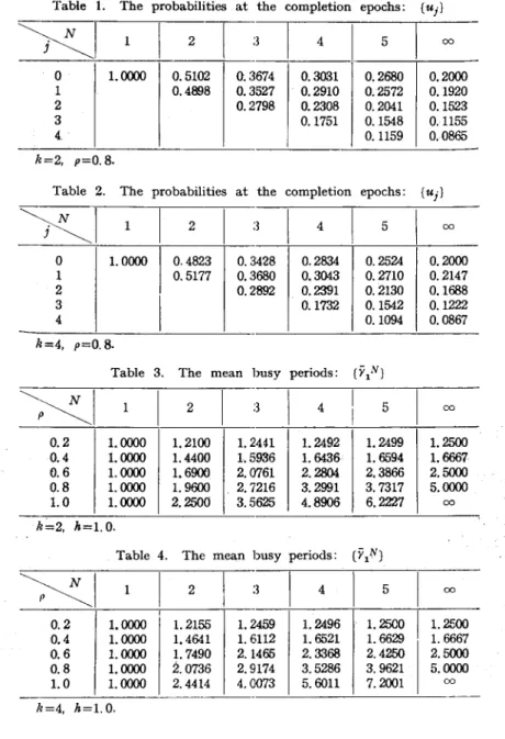
First, for comparison, we calculate the steady-state probabilities of the number of customers in the system at the service completion epochs by using the imbedded Markov chain method. In the examples, only the case where the service time distribution is k-Erlang distribution is calculated. Table 1 shows the steady-state probabilities at the service completion epochs for the case of k=2 and Table 2 shows those for the case of k=4, while p is fixed to O.s.

In the tables, the columns which correspond to N =00 show the

probabilities for M

/Ek/l

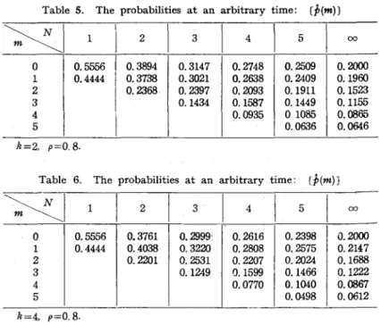
with infinite waiting room. Table 3 and Table 4 show the mean busy periods.

Using the values in Table 3 and Table 4, we can calculate the probabilities at an arbitrary time under the steady state, which are

(21)

Table 1. The probabilities at the completion epochs: {Uj}

}Zl

o

1 2 3 4 1 1.0000 k=2, p=0.8. 2 0.5102 0.4898 0.3 0.3 0.2 674 527 798 4 5 00 0.3031 0.2680 0.2000 0.2910 0.2572 0.1920 0.2308 0.2041 0.1523 0.1751 0.1548 0.1155 0.1159 0.0865

Table 2. The probabilities at the completion epochs: {Uj}

~I

1 2 4 5 0 1. 0000

I

0.4823 0.3428 0.2834 0.2524 1 0.5177 0.3680 0.3043 0.2710 2 0.2892 0.2391 0.2130 3

I

0.1732 0.1542 4 0.1094 k=4, p=0.8.

Table 3. The mean busy periods: {YIN}

XI

2 4 5 -0.2 1. 0000 1. 2100 1.2441 1. 2492 1. 2499 0.4 1. 0000 1. 4400 1. 5936 1. 6436 1. 6594 0.6 1. 0000 1.6900 2.0761 2.2804 2.3866 0.8 1. 0000 1.9600 2. 7216 3.2991 3.7317 1.0 1.0000 2.2500 3.5625 4.8906 6.2227 k=2, h=l.O.

Table 4. The mean busy periods: {YIN}

XI

2 I 0.2 1.0000 1. 2155 1. 0.4 1. 0000 1.4641 1. 0.6 1. 0000 1. 7490 2. 0.8 1. 0000 2.0736 2. 1.0 1. 0000 2.4414 4. k=4, h=l. O. 2459 6 112 1 465 9 174 00 73 4 5 1. 2496 1. 2500 1. 6521 1. 6629 2.3368 2.4250 3.5286 3.9621 5.6011 7.2001 00 0.2000 0.2147 0.1688 0.1222 0.0867 00 1. 2500 1. 6667 2.5000 5.0000 00 00

I

1.2500 _1.₆₆₆₇ 2.5000 5.0000 00

(22)

Table 5. The probabilities at an arbitrary time: (p(m)}

~I

1 2 3 4 5 00 0 0.5556 0.3894 0.3147 0.2748 0.2509 0.2000 1 0.4444 0.3738 0.3021 0.2638 0.2409 0.1960 2 0.2368 0.2397 0.2093 0.1911 0.1523 3 0.1434 0.1587 0.1449 0.1155 4 0.0935 01085 0.0865 5 0.0636 0.0646 k=2, p=0.8.

Table 6. The probabilities at an arbitrary time: (p(m)}

~I

1 2 3 4 5 00 0 0.5556 0.3761 0.2999' 0.2616 0,2398 0.2000 1 0.4444 0 .. 4038 0.3220 0.2808 0.2575 0.2147 2 0.2201 0.2531 0.2207 0.2024 0.1688 3 0.1249 O. 1599 0.1466 0.1222 4 0.0770 0.1040 0.0867 5 0.0498 0.0612 k=4, p=0.8.

shown in Table 5 and Table 6.

In practice, we have often estimated the capacity of the buffer storage on the assumption that the probability of overflow is nearly equal to the probability thl;lt a departing customer leaves behind more customers than the capacity. In the tables, the probability that a departing customer leaves behind more than 5 customers is 0.2537 (k= 2) or 0.2076 (k=4) for the M/Ek/1 model with infinite capacity. On the other hand, the probability that an arriving customer finds the waiting room full is 0.0636 (k=2) or 0.0498 (k=4) for the M/Ek/1 model with finite capacity (N =5), Therefore, when N is small, we overesti-mate the capacity of the buffer storage by using the M/Eh/1 model with infinite capacity.

(23)

On the Busy Period in the Queueing System 137

Acknowledgment

The author is deeply indebted to the refrees who pointed out some faults in equations and suggested numerous improvements throughout the paper.

References

(1] Cohen, ].W., The Single Server QueHe, North-Holland, 1969.

(2] Brockmeyer, B., H.L. Halstrom and A. ]ensen, "The Life and Works of A.K. Erlang," Trans. Dan. A cad. Tech. Sci., No. 2 (1948).

[3] Finch, P.D., "The Effect of the Size of the Waiting Room on a Simple Queue,"

J. Ray. Statist. Soc., B-20 (1958), 182-186.

[ 4] Finch, P.D., "On the Transient Behavior of a Queueing System with Bulk Service and Finite Capacity," Annals. Math. Statist., 33, 3 (1962), 973-985. [5] lain, H.C., "Queueing Problem with Limited Waiting Space," Nav. Res. Log.

Quart., 9, 3 & 4 (1962). 245-252.

[6] ] aiswal, N.K., Priority. Queues, Academic Press, 1968.

[7] Keilson,]., "The Ergodic Queue Length Distribution for Queueing System with Finite Capacity," J. Ray. Statist. Soc., B-28, 1 (1966), 190-201. [8] Riordan, ]., Stochastic Service Systems, John Wiley, 1962.