遲画ｸｩ邉ｻ蜿翫豐ｸ鬨ｰ邉ｻ縺ｫ縺翫¢繧区ｰ玲ｳ｡髢灘ｹｲ貂峨蜍慕噪繝｢繝Ν

修 士 論 文

Dynamical models of bubble-bubble interactions

in isothermal and boiling systems

等温系及び沸騰系における気泡間干渉の動的モデル

1 - 50

ページ 完

平成

16

年

2

月

13

日 提出

指導教官

庄司 正弘 教授

Master’s Thesis

Dynamical Models

of

Bubble-bubble Interactions

in

Isothermal and Boiling Systems

by

Manabu Tange

Department of Mechanical Engineering,

Graduate School of Engineering

Abstract

This master’s thesis examines the essences of the interactions between gen-erated bubbles in isothermal system and boiling system.

In isothermal system, gas bubbles were generated from twin orifices sub-merged in water. Bubbling features were observed using high-speed video. At each orifice, a hot wire anemometer detected the micro-convection in-duced by successively generated bubbles. It is found that bubbling pattern differs depending on the chamber volume as well as the air volumetric flow rate. When the chamber volume is small and the flow rate is relatively low, “reciprocal” and “counterpart” bubbling patterns repeatedly appear with gradual decreasing the air flow rate. Between the two patterns, “aperiodic” bubbling takes place. To reveal the mechanism of such interactive bubbling features, a simplified theoretical model is proposed. It describes the time evolution of individual bubble volume basing on the equations of motion for gas and liquid. The distribution of air flow into two bubbles is uneven and yields various bubbling patterns. The model explains well the appearance of three bubbling patterns and their repetition.

In boiling system, vapor bubbles were generated from two nucleation sites on an artificial surface. Experiment revealed that average bubbling frequency and bubbling periods distribution changed if a cavity spacing, an intensity of the interaction, was varied. In order to reproduce and understand the interaction, a simple dynamical model similar to that in isothermal system, was constructed. It describes the temperature, bubble volume and previ-ous bubble motion on each site. Nevertheless it made the bubbling periods distribution, clear dependence of cavity spacing is not shown. Further im-provements of the model are required.

Acknowledgment

I sincerely express gratitude to prof. Masahiro Shoji, my supervisor, for his generous help in preparing this thesis. When I worried myself too much over my future specialty I would major in, I read a essay [1] written by him in a journal. In the essay, he said that engineering researchers should study more individually and more easily. I was moved to action by what he said, and chose to study under him in my master’s course.

I would also like to acknowledge prof. Shigeo Maruyama for his helpful and piercing comments at research meetings. His penetrating comments pointed out where the problem of my model was and helped me strike out in new directions.

I would like to acknowledge with much thanks Dr. Zhang and Mr. Shimura for their fantastic experimental results which gave me impulses of modeling. I would like to appreciate Mr. Watanabe and Mr. Miyazaki for their kind help in performing the experiment and Dr. Matsumoto at AIST (national institute of advanced industrial science and technology) for fabrica-tion of cavities on silicon surfaces. I could not have conducted all experiments without their helps.

Hearty gratitude should be expressed to the members of our laboratory, especially Dr. Ito, Dr. Shibuta and Mr. Miyauchi, who have discussed all things of research and study.

Finally I am most indebted to my parents who have supported my living and my dreams.

Contents

Nomenclature . . . 8

1 Introduction 10 1.1 Introduction of Nucleate Boiling . . . 10

1.2 Introduction of Interaction . . . 11

1.3 Dynamical Behavior of Boiling . . . 13

1.4 Past Researches of Artificial Surface in Our Laboratory . . . . 14

1.5 Objectives . . . 15

2 Interaction in Isothermal System 16 2.1 Introduction . . . 16

2.2 Experimental Apparatus . . . 17

2.3 Experimental Results . . . 18

2.3.1 Bubbling pattern at low flow rate . . . 18

2.3.2 Pattern transition . . . 21

2.3.3 Power law for pattern transition . . . 22

2.4 Simplified Theoretical Model . . . 22

2.4.1 Assumptions . . . 22

2.4.2 Phenomenological governing equations . . . 24

2.5 Model Behavior . . . 25

2.5.1 Configuration space and phase space . . . 25

2.5.2 Effect of surface tension . . . 26

2.5.3 Effect of inertial force . . . 27

2.5.4 Growth of twin bubbles and trajectory on configura-tion space . . . 28

2.5.5 Simulated spectrogram and power law . . . 29

2.6 Concluding Remarks . . . 29

3 Interaction in Boiling System 32 3.1 Introduction . . . 32

3.2 Experimental Setups . . . 33

3.3.1 Bubbling frequency[26] . . . 33

3.3.2 Distribution of bubbling periods . . . 34

3.3.3 Photographic observation . . . 35

3.4 Simplified Theoretical Model . . . 37

3.4.1 Problem statement . . . 37

3.4.2 Assumptions . . . 38

3.4.3 Phenomenological governing equation . . . 42

3.5 Model Behavior . . . 42

3.6 Concluding Remarks . . . 44

4 Conclusion 45

List of Figures

1.1 Boiling curve [2]. . . 11

1.2 Analogy of bubbling between isothermal system and boiling system. . . 12

1.3 Actual boiling surface and interaction. . . 12

1.4 Analogy of bubble-bubble interactions between isothermal sys-tem and boiling syssys-tem. . . 13

1.5 Coupled map lattice of boiling [10] . . . 14

2.1 Sketch of experimental setups . . . 18

2.2 Snapshots of major bubbling patterns. . . 19

2.3 Time series of bubble volume and power spectrum of each bubbling pattern. . . 20

2.4 Spectrogram of wire probe signal. . . 21

2.5 Flowrate at pattern transition(experiment). . . 22

2.6 Sketch and notation of idealized bubble shape . . . 23

2.7 A typical example of trajectory on configuration space. . . 26

2.8 A typical example of trajectory on phase space. . . 27

2.9 Pressure difference with surface tension. . . 28

2.10 Time series of bubble volumes and phase space expression. . . 29

2.11 Spectrogram of simulation results. . . 30

2.12 Flow rate at pattern transition of simulation results. . . 30

3.1 Schematic diagram of experimental system of nucleate pool boiling on artificial surface . . . 34

3.2 Bubbling frequency and three dominant factors . . . 35

3.3 Bubbling period distribution (Experiment) . . . 36

3.4 Vertical coalescence . . . 36

3.5 Horizontal coalescence. . . 37

3.6 Declining coalescence . . . 37

3.7 Notation of bubble condition . . . 39

Nomenclature

cp: specific heat at constant pressure, J/Kg K

D : diameter, m f : force, N

Fo := αt/L2_{, Fourier number, –}

g : gravitational acceleration, m/s2 h : heat transfer coefficient, W/m2K

hfg : enthalpy of vaporization, J/kg Ja := ρ`cp,`∆T /ρvhfg, Jacob number, – k : thermal conductivity, W/mK Lc:= p σ/(ρ`− ρv)g, capillary length, m Nu := hL/k, Nusselt number, – P : pressure, Pa Pr := ν/α, Prandtl number, –

q : volumetric gas flow rate in chap. 2, m3_/s, heat flux in chap. 3, W/m2

r : bubble radius of curvature, m

S : spacing between orifices in chap. 2, m

spacing between cavities in chap. 3, m

T : temperature, K t : time, s

u : velocity, m/s V : bubble volume, m3

Greek letters

α : thermal diffusivity, m2_/s

δ : thickness of orifice, m

δth: thickness of superheated liquid layer, m

γ : width of temperature distribution θ := sin−1(D/2r), rad

µ : viscosity, Pa · s

ν : dynamical viscosity, m2_/s

ρ : density, kg/m3

σ : surface tension, N/m

Subscripts on any variable, Q:

Qc: value for chamber

Qd: value for detachment

Qi : value for orifice i in chap. 2 and site i in chap. 3 (i = 1, 2)

Qg : value for gas

Q` : value for liquid

Qv: value for vapor

Qpre: value for previous bubble

Qwake: value for wake Superscripts on any variable, Q:

¯

Q : mean value of Q

˙

Q : time derivative of Q

¨

Q : second time derivative of Q Q∗ _{: dimensionless value of Q}

Chapter 1. Introduction

Chapter 1

Introduction

1.1

Introduction of Nucleate Boiling

Nucleate boiling has been extensively utilized in industry in view of the fact that it is one of the most efficient heat transfer modes, particularly in high energy density systems, such as nuclear power plants, boiler and the like. These conventional applications intensely need the useful correlation func-tions like ¯q = f ( ¯T ), namely “boiling curve” as shown in Fig. 1.1[2]. Here, ¯q

and ¯T are average heat flux and average surface temperature, respectively. In

other words, all correlations took the average properties in time and in space. Heat transfer of nucleate boiling is correlated mainly from experiments due to highly nonlinear behavior of vapor bubble while some other convectional flows correlated from analytical methods [3].

In recent years, however, the spatio-temporal (in space and in time) un-derstanding of boiling behavior has come to be required (Shoji [4] proposed a vision of “boiling chaos”). Cooling of a recent electric device with boiling heat transfer will be required for its large heat generation since air cooling is not enough to maintain the temperature of the devices. Traditional boiling researches paying attention to average heat transfer properties cannot give sufficient solutions since the size of the cooled surface is comparable with bubble radius and heat transfer become highly transitional.

One of the techniques to facilitate the interaction of boiling is to separate the complexities into hydrodynamical part and thermal part. In other words, It is effectual to investigate bubble dynamics and its interaction of gas-liquid system without phase change, isothermal system. Takagi and Shoji [5] pre-sented an analogy of bubble behavior between isothermal and boiling system. Heat flux and surface temperature in boiling system correspond to gas flow rate and chamber pressure in isothermal system.

Chapter 1. Introduction

Figure 1.1: Boiling curve [2].

1.2

Introduction of Interaction

Particular discussions of isothermal and boiling systems are mentioned in each chapter.

A conceptual sketches of actual boiling surface was illustrated in Fig. 1.3. Some theoretical studies have discussed only single bubble behaviors for several decades while collections of correlations have governed the boiling research field. Some recent experimental researches revealed that chaos rules in bubbling of boiling and isothermal system and it results from interaction between bubbles [6].

As already stated, the scopes of conventional boiling researches have been an average properties of whole surface. The reason why such approach have been taken is that an actual surface has randomly distributed nucleation sites which play the nucleation of vapor bubble and it is difficult to extract the fundamental process like single site dynamics. A recent micro-fabrication technology enables us to pick up the single bubble behavior. Takagi et al. [7] investigate experimentally and theoretically a behavior of a boiling bubble from a micro-scale heater. They evaluate fractions of heat quantity released

Chapter 1. Introduction Orifice Previous bubble Air bubble Gas chamber Orifice plate Cf. Bubbling from a nozzle Gas flow Heated surface Superheated liquid layer Cavity Previous bubble Vapor bubble Heat flux Wake effect of previous bubble Vaporization

Bubbling in isothermal system. Bubbling in boiling system.

Figure 1.2: Analogy of bubbling between isothermal system and boiling sys-tem. Bubble in bulk Average properties, T, q Heat flux Actual surface Single bubble Nucleation site interaction Nucleation site (Instantaneous conditions, T(x, t), q(x, t) )

Figure 1.3: Actual boiling surface and interaction.

through different paths: vaporization, induced flow and natural convection. In contrast, many researches of isothermal system have studied bubble dy-namics in bulk liquid. Heat transfer from heated surface, however, is influ-enced by a great deal by bubble behavior near the surface. This evidence is helpful to construct model in chapter 3 since we can consider small volume near the surface.

Chapter 1. Introduction

Flow distribution Bubble induced flow

Temperature distribution Convection

(Bubble induced flow)

Bubbling from two orifices. Nucleate boiling on two cavities.

Figure 1.4: Analogy of bubble-bubble interactions between isothermal system and boiling system.

interaction. Isothermal system and boiling system with two bubbling sources are sketched in Fig. 1.4. Pressure of a chamber and superheat of heated surface drive the bubbling in isothermal and boiling system, respectively. Distributions of gas flow or heat flux cause interactions.

The difference, however, was pointed out by considering the governing equations of two systems. Hydrodynamical interaction was governed by equa-tions of moequa-tions of liquid and gas which define second time derivatives of the quantities and remind us a concept of “inertia”. In contrast, Thermal inter-action, a conduction, was governed by diffusion equations which determine first time derivatives of quantities.

1.3

Dynamical Behavior of Boiling

Hardenberg [8] et al. investigated experimentally the dynamics of boiling, especially nucleation site interaction using statistical analysis.

Numerical simulation of boiling is still unrevealed field due to interfa-cial phenomena. For example, discontinuity of interface structure, namely vapor bubble coalescence, and vaporization coefficient have been ambiguous yet. One of few researches, a study by Dhir [9], solved the conservation equation of mass, momentum and energy for the liquid and vapor phase simultaneously with the continuously evolving of the interface at and near a heated surface. The simulation results of the bubble behaviors showed good agreement with the experimental data. In this simulation, however, the temperature of heated surface was assumed to be constant.

There are few dynamical model of boiling as follows. Yanagita [10] em-ployed coupled map lattice (CML, see an overview of CML by Kaneko [11]) to simulate boiling regimes, nucleate boiling and film boiling as shown in

Chapter 1. Introduction

Nucleate boiling. Film boiling.

Figure 1.5: Coupled map lattice of boiling [10]. (These figures were recon-structed by the author).

Fig. 1.5. There is large degrees of freedom, number of meshes. The mesh was heated from below and cooled from top Darkness mean temperature and lamb of black lattices meaning bubbles feel buoyancy. It is a dynami-cal system with continuous field variables but with discrete space and time. It reproduce transition between nucleate boiling and film boiling by setting only several simple rules, conduction and buoyancy.

In contrast, Ellepola and Kenning [12] proposed a simplified dynamical model of an interaction between two nucleation sites only with three degrees of freedom, temperatures of two sites and an intervening wall. The time evolution of the model was based on conduction between each site and in-tervening wall, vaporization from each site and convective heat transfer from intervening wall. They illustrated that time series of temperature became chaotic or periodic depending on input heat flux. In this model, chaos comes from switching of vaporization (see the detail in his Ph.D thesis [13]).

1.4

Past Researches of Artificial Surface in

Our Laboratory

Researches of nucleate boiling on artificial surface in our laboratory have started with boiling from a single cavity [14] by Shoji and Takagi. They ex-amined the effects of cavity shapes: conical, cylindrical and reentrant. Yasui and Yokota performed the experiments in various conditions of diameters and depths of a cavity and a spacing between cavities (reviewed in Shoji [15]). Zhang and Shoji compiled these experiments and evaluated the interaction as reviewed in section 3.3. Surapong [16] performed the experiments of triple

Chapter 1. Introduction cavities and analysis as Zhang and Shoji.

1.5

Objectives

There are models of two types: models for prediction and models for un-derstanding. Numerical simulations and empirical correlations belong to the former. While they are very effective in engineering, they cannot grow our understanding well sometimes, especially for dynamical phenomena or inter-actions, even though they reproduce some curious experimental results.

In this master’s thesis, the author proposed two simplified dynamical models for understandings of bubble-bubble interactions in isothermal and boiling systems. “Simplified” means number of variables, degrees of freedom, is not large and each variables are physically meaningful. These models were constructed in the form of deterministic dynamical systems, ˙x = f (x), like a Lorenz model [17] which is simplified model of two dimensional Navier-Stokes equation under the condition as benard convection and behaves non-periodically only with three variables.

In chapter 2, bubbling from submerged twin orifices with a common plenum was dealt with. When the plenum volume is relatively small and a flow rate was extremely low, the bubbling from two orifices strongly inter-acts each other. Observation of bubbling and measurement of flow induced by bubble was conduct experimentally. A simplified mathematical model which describe time evolution of bubbles volumes is proposed and it reveals the mechanism of bubble-bubble interaction.

Taking a liking for results in isothermal system, the author attempt to construct a dynamical model of boiling bubble behavior on artificial surface and their interaction in chapter 3. As mentioned in subsection 1.2, interaction in boiling system become more difficult than isothermal system. Therefore more degrees of freedom is needed and it is ambiguous to understand even qualitatively.

Chapter 2. Interaction in Isothermal System

Chapter 2

Interaction in Isothermal

System

2.1

Introduction

Bubble formation has been widely used in industry such as chemical plants, bubble towers and the like. It is also an important physical process in boiling phenomena. To achieve a better comprehension about the bubble dynamics, numerous researches have been attempted in the past by focusing on bubble generation, growth and detachment (e.g., Clift et al. [18]). Most researches have had target on a single isolated bubble because the interaction between successively generated bubbles or adjacent bubbles is rather complex and difficult to deal with due to its strongly nonlinear nature. Thus the interactive aspects have been excluded from the consideration for long period by taking the average in time or in space. In many actual systems of utilizing bubbles, however, it is usual for multiple bubbles to appear. So the bubble-bubble interaction as well as bubble-liquid interaction is the essential issue, and some recent researches deal with such problem.

In a system of air bubble generation from a single nozzle in water, Mit-toni et al. [19] and Tritton and Egdell [20] obtained time series of pressure signals at upstream nozzle or flow velocities near the nozzle exit. Then they carried out nonlinear analysis for the data, showing that some chaotic dy-namics exists in the system. Shoji [21] observed period doubling bifurcation in departing bubble frequency of a chain of air bubbles generated from a single orifice submerged in water, and Zhang and Shoji [22] succeeded to explain the phenomena by proposing a nonlinear model which considers the interactive effects of the preceding bubble. In contrast, there are only a few researches available for the systems of multiple orifices. Titomanlio et al. [23]

Chapter 2. Interaction in Isothermal System conducted an experiment of bubbling from two orifices connected to a com-mon chamber, and found that at high air flow rate, the detachment bubble volume is almost equal to that of a single orifice system having a half cham-ber volume in half flow rate. In a similar system, Ruzicka et al. [24] measured the pressure signal inside the chamber and found that the signal shows two different fluctuation structures “synchronous” and “asynchronous”, depend-ing on the air flow rate. They also discussed nonlinear characteristics and its dependence on various control parameters. To our knowledge, there is no available model or theoretical approach to comprehend the interaction between bubble and bubble or between bubble and liquid.

This chapter describes the results of experimental and theoretical study performed to understand bubbling behaviors from submerged twin orifices that interact each other through a common chamber. In the experiment, bubbling feature was precisely specified varying gas flow rate. It is found that at relatively low flow rate, various bubbling patterns appear repeatedly in a complex manner. To reveal the mechanism of such pattern appearance and transition, a simplified theoretical model is proposed. This model describes the time evolution of bubble volume at each orifice basing on equation of motion for liquid and gas, which explains well the experimental results.

2.2

Experimental Apparatus

Fig. 2.1 shows the experimental apparatus schematically. Air and pure water were used as the test fluids. The air was supplied to the chamber under a constant flow rate by a compressor through a flow meter and a fine brass cap-illary tube of 0.3mm in inner diameter and 137mm in length. The capcap-illary tube was served to maintain a constant flow rate condition. Bubbles were generated into a stagnant water pool from two cylindrical orifices of 2mm in diameter. The orifices were fabricated on a 1mm-thick, 60mm-diameter brass plate, which constitutes the top side-wall of the chamber.

The spacing between orifices plays an essential role in the effectiveness of interaction between generated bubbles. In general, the interaction involves two interactive processes: one through the liquid and the other through the chamber. In this study, in order to simplify the system, the spacing between orifices was taken large enough to be able to ignore the effects of interaction through liquid. Namely, attention was paid only to the interaction through the common chamber. According to the past researches of nucleate boiling (e.g., Calka and Judd [25] and Zhang and Shoji [26]), the interaction between horizontally-adjacent bubbles is negligible when the spacing between the nu-cleation sites is larger than three times of the bubble departure diameter. The

Chapter 2. Interaction in Isothermal System Chamber C o mp re sso r Orifices H o t F ilm P ro be H o t F ilm P ro be W a ter P oo l

Capillary Tube Flo

w

Me

ter

High-speed Video Camera

Figure 2.1: Sketch of experimental setups

critical spacing of this becomes 15mm in the present experiment because the bubble departure diameter was mostly around 5mm. So the spacing of 30mm employed in the present experiment is well expected to satisfy the condition,

including a surplus. In the experiment, the chamber volume, Vc as well as

the gas flow rate, q, was varied in a wide range. The following discussion, however, is restricted within a condition of Vc = 10m` which the interaction become vivid.

Bubbling behaviors were observed by a high speed video camera with 1000 frames/s. A hot film probe was set at the vicinity of each orifice to detect liquid flow (micro convection) induced by generated bubbles. The location of the probe was 0.5mm height from the orifice plate and 3mm horizontal distance from the orifice center, which was determined from repeated prelim-inary tests to obtain maximum signal and to correspond well to the bubble generation, growth and departure. Thus the signal output becomes a good indicator of bubbling features, providing valuable information to diagnose the linearity or complexity of bubble generation and interaction.

2.3

Experimental Results

2.3.1

Bubbling pattern at low flow rate

In the present experiment, various types of bubbling patterns were observed, depending on the chamber volume as well as the air flow rate. Three types of bubbling patterns appear at relatively low flow rate. For each typical cases, the snapshot in Fig. 2.2 and time series of bubble volumes in Fig 2.3 are obtained from high speed movies, and the power spectrum calculated from

Chapter 2. Interaction in Isothermal System Orifice 1 Orifice 2

R

C

A

the signal of hot wire probe.

1 (Reciprocal bubbling) Bubbles are generated from each orifice recip-rocally (Fig. 2.2–(1)). Once a bubble departs from the one orifice, the next bubble is generated and departs from the other orifice. Since the air may be supplied evenly in time to both orifice, fundamental frequency of bubble de-parture in this case becomes f = q/2 ¯Vd, where ¯Vd is the averaged departure bubble volume (Fig. 2.3–(1)).

2 (Counterpart bubbling) Bubbles are generated from either of the ori-fices (Fig. 2.2–(2)). So the fundamental frequency in this case is f = q/ ¯Vd, which is twice as large as that of reciprocal bubbling (Fig. 2.3–(2)).

3 (Aperiodic bubbling) This pattern does not belong to neither of the two patterns above mentioned (Fig. 2.2–(3)). Namely, several bubbles sub-sequently generate from either of the orifices but the active orifice changes from one to the other in a random manner (Fig. 2.3–(3)).

In any of the above-mentioned three patterns, bubbles synchronously start to grow from both orifices at the first stage of bubble generation. How-ever, at the moment when the bubbles reach to a certain critical size, one bubble continues to grow while the other bubble stop to grow and diminishes to finally disappear.

Chapter 2. Interaction in Isothermal System 0 20 40 60 80 0 50 100 150 200 250 300 Bubble Volumes, V i (10 -3 ml) Time, t(ms) Orifice 1 Orifice 2 0 10 20 30 40 50 Intensity(dB) Frequency, f(Hz) Orifice 1 Orifice 2 (1) Reciprocal bubbling (q = 1.6 ml/s). 0 20 40 60 80 0 50 100 150 200 250 300 Bubble Volumes, V i (10 -3 ml) Time, t(ms) Orifice 1 Orifice 2 0 10 20 30 40 50 Intensity(dB) Frequency, f(Hz) Orifice 1 Orifice 2 (2) Counterpart bubbling (q = 1.3 ml/s). 0 20 40 60 80 0 50 100 150 200 250 300 Bubble Volumes, V i (10 -3 ml) Time, t(ms) Orifice 1 Orifice 2 0 10 20 30 40 50 Intensity(dB) Frequency, f(Hz) Orifice 1 Orifice 2 (3) Aperiodic bubbling (q = 1.35 ml/s).

Figure 2.3: Time series of bubble volume and power spectrum of each bub-bling pattern.

Chapter 2. Interaction in Isothermal System 0 10 20 30 40 50 0.4 0.6 0.8 1 1.2 1.4 1.6 1.8 2 Frequency, f(Hz)

Gas Flow Rate, q(ml/s) Orifice 1 0 10 20 30 40 50 0.4 0.6 0.8 1 1.2 1.4 1.6 1.8 2 Frequency, f(Hz)

Gas Flow Rate, q(ml/s) Orifice 2

Figure 2.4: Spectrogram of wire probe signal.

2.3.2

Pattern transition

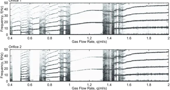
To obtain better matching between the air flow rate and the bubbling pat-terns and also to observe precisely the transition from one pattern to the other, the special test was conducted by gradually decreasing the air flow rate. This was a transient experiment but the decreasing rate of air flow was very slow at an order less than 0.01m`/s, so it may be said that the data ob-tained were of quasi steady state. Fig. 2.4 shows the spectrograms obob-tained from the hot wire probe signal of each orifice, in which the strength of the power (scale of the amplitude) of Fourier analysis is illustrated in colored for every signal-detected flow rate.

The region of air flow rates where clear peaks of frequency appear at both orifices corresponds to the periodic bubbling, and the region with no clear peaks to “aperiodic” bubbling. In the region of “counterpart” bubbling, a stripe appears only at an active orifice whereas in the region of “reciprocal” bubbling, stripes appear in both spectrograms for the two orifices. The fundamental frequency (i.e. the lowest peak) of “reciprocal” bubbling is lower than that of “counterpart” bubbling because the air flow is splitted to both orifice in time-avarage sense. The most interesting and important information that Fig. 2.4 provides is that a set of regions of air flow rate, where the two periodical patterns appear and aperiodic pattern exists in between, appear repeatedly in a wide range of air flow rate.

Chapter 2. Interaction in Isothermal System 0.25 0.5 1 2 1 2 3 4 5 6 Flow Rate, q(ml/s)

Appearance Order of Transition, n

Figure 2.5: Flowrate at pattern transition(experiment).

2.3.3

Power law for pattern transition

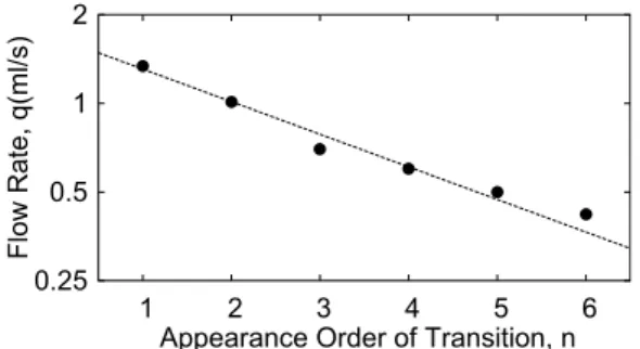
The values of air flow rate, qc,n, at which the set of the combined pattern region appears are plotted in Fig. 2.5 as a function of the order of the ap-pearance, n. The data is well correlated by the following equation:

qc,n = 1.68 exp(−0.255n) (2.1)

This result clearly indicates the existence of a power law, suggesting that some nonlinear chaotic dynamics exists in this system.

2.4

Simplified Theoretical Model

2.4.1

Assumptions

In order to reveal the physical mechanisms of bubbling features described in the previous section, especially the appearance, transition and repetition of bubbling patterns, a simplified model is constructed to describe bubble generation at each orifice. In this modeling, bubble volume at each orifice,

V1 and V2, are taken as a couple of variables, and the local pressure at the inlet of each orifice is considered. The fluctuation of the pressure connects to the instantaneous variation of each variable (each bubble volume). The main issue concerned here is to make clear the physical process how the distribution of air supplied into two orifices is determined and why it becomes uneven, which may finally yield complex bubbling features. Since the present system is symmetry with respect to two orifices, the governing equations of the model should be written in the form as

½ _¨

V1 = f (V1, V2, ˙V1, ˙V2; q) ¨

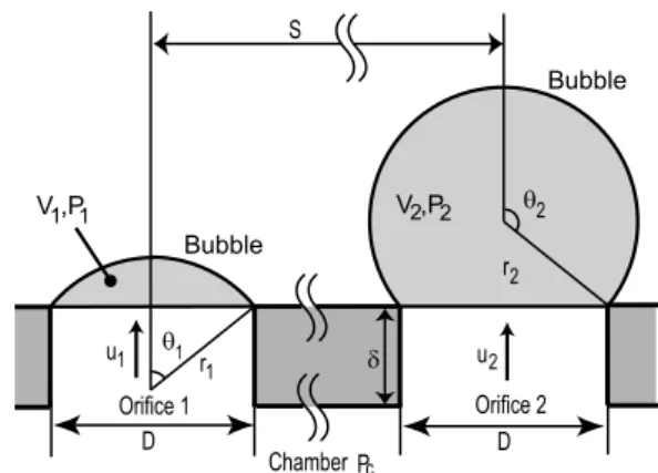
Chapter 2. Interaction in Isothermal System r D S 1 2 r 2 1 D u₁ u₂ c P Orifice 1 Orifice 2 Chamber θ θ δ V ,P_{1 1} V ,P_{2 2} Bubble Bubble

Figure 2.6: Sketch and notation of idealized bubble shape

Here q is the volumetric air flow rate supplied into the chamber. In the present model, q is a parameter but is considered to be constant in time.

For simplicity, the followings are assumed:

Assumption 2.1 The bubble shape is a sectional part of a sphere as shown in Fig. 2.6. So the instantaneous bubble volume and radius of curvature of the bubble are respectively expressed as follows:

Vi(ri) = πr3 i 3 (cos 3_θ i− 3 cos θi+ 2) (2.3) ri = D 2 sin θi . (2.4)

Assumption 2.2 Properties of air and water are constant. This assumption includes the incompressibility of air as well as water.

Assumption 2.3 The viscous effects of liquid motion are negligible.

Assumption 2.4 The inertia effects of gas flow in bubble growth are negli-gible.

Assumption 2.5 The bubble departure volume is determined from the force balance between buoyancy and surface tension as follows:

Vd =

σπD

(ρ`− ρg)g

Chapter 2. Interaction in Isothermal System After the bubble departs from the orifice with the value of Eq.(5), the next following bubble is assumed to start growing from zero volume. This as-sumption is a nonlinear on–off condition but it is noted that the continuity of variables and that of its time derivative hold except the volume at the instant of detachment.

Assumption 2.6 The volumetric air flow rate into the chamber is constant. This assumption together with Assumption 2.2 indicates that the total air flow rate supplied to the twin orifices is constant. This condition can be written in the following forms:

˙

V1+ ˙V2 = q (Const.) (2.6)

¨

V1+ ¨V2 = f1+ f2 = 0. (2.7)

The interaction between bubbles generated from two orifices is restricted by the conditions of Eqs.(2.6) and (2.7).

Assumption 2.7 There is no pressure drop inside the passage of the orifice. In general, equation of motion of gas inside the orifice can be written as

∂ui ∂t = − 1 ρg ∂P ∂x − ui ∂ui ∂x + νg ∂2_u i ∂x2 (i = 1, 2). (2.8)

By integrating Eq.(2.8) with respect to x (flow direction), the Assumption 2.3 yields δ∂ui ∂t = 1 ρg (Pc− Pi) (i = 1, 2). (2.9)

Noting that Aui = ˙Vi, Eq.(2.9) can be rewritten for the bubble volume as ¨

Vi =

A ρgδ

(Pc− Pi) (i = 1, 2). (2.10)

2.4.2

Phenomenological governing equations

In order to complete the model formulation, instantaneous pressure inside the growing bubble must be considered. As well known as the Rayleigh-Plesset equation (e.g. Plesset and Prosperetti [27]), the equation of motion of liquid around a spherical bubble is given by

P = 2σ r + ρ`(r¨r + 3 2˙r 2<sub>) +</sub> 4µ` r ˙r. (2.11)

Here, P is the excess pressure from that of liquid far from the bubble. The terms of right hand side of Eq.(2.11) represent surface tension, inertial force

Chapter 2. Interaction in Isothermal System and viscous force, respectively. Laplace pressure is often used for measure-ment of surface tension [28] 1_{. If we rewrite Eq.(2.11) by taking the bubble} volume as the variable in place of r, we can learn with ease that inertial

and viscous terms in Eq.(2.11) relate to ˙V2 _{and ˙V respectively. So from}

Eq.(2.11) together with the Assumption 2.1, the pressure inside the bubble may approximately be expressed in the following form:

Pi = 2σ

ri

+ β ˙V_i2 (i = 1, 2). (2.12)

In deriving Eq.(2.12), it is assumed that the coefficient of inertia term, β,

is constant. By substituting Eq.(2.12) into Eq.(2.10) and by eliminating Pc

using the relation of Eq.(2.7), the following set of governing equations are

obtained:        ¨ V1 = A 2ρgδ (P2− P1) ¨ V2 = A 2ρgδ (P1− P2), (2.13) where Pi = 2σ ri + β ˙V2 i (i = 1, 2). (2.14)

2.5

Model Behavior

Basing on the present model, the simulation was performed using the gov-erning equations of Eqs.(2.13) and (2.14). The constants involved in the equations are A/(ρgδ) = 9.52 × 10−5 and β = 5 × 1011 for the present exper-imental conditions.

2.5.1

Configuration space and phase space

Configuration space is a mathematical space easy to discuss the dynamic behaviors of a physical system. The configuration space of the present case

can be constructed by taking bubble volumes, V1 and V2, as coordinates.

On this space, an instantaneous state of the twin bubbles is expressed by

the point (V1, V2), and the time evolution of the state by the movement

(trajectory) of the point. The trajectory is determined by Eq.(2.13). A typical example of the trajectory is shown in Fig. 2.7 by a thin solid curve, which indicates the bubble volume time-development starting from a certain

1_{Few people are aware that one of its pioneers was a young physicist named Erwin}

Chapter 2. Interaction in Isothermal System 0 10 20 30 40 0 10 20 30 40 Bubble Volume at Orifice 2 , V2 (1 0 -3 ml )

Bubble Volume at Orifice 1, V₁ (10-3ml)

V =V , Bubble at Orifice 2 departs_{2 d}

V =V , Bubble at Orifice 1 d e p arts 1 d r =r , V = V , u nstable 1 2 1 2 r =r , V =V , stable 1 2 1 2 \ (a) (b) 0 2 4 6 8 0 2 4 6 8 Bubble Volume at Orifice 2 , V2 (1 0 -3 ml )

Bubble Volume at Orifice 1, V₁ (10-3ml)

r =r , V =V , uns table 1 2 1 2 r =r , V = V , stable 1 2 1 2 \ Trajectory r =r , V =V , stable1 2 1 2 (b) B A1 A2 C

Figure 2.7: A typical example of trajectory on configuration space.

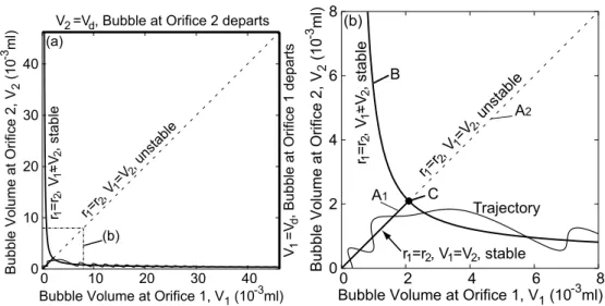
initial condition under the air flow rate of q = 1.0m`/s. Since the total air flow rate supplied to the twin orifices is constant (Assumption-2.6), the point on the trajectory moves at a constant speed in the upper-right direction while at the velocity determined by Eqs.(2.13) and (2.14) in the upper-left direction. The time variation of bubbles state is much easily understand on phase space. As the total air flow rate supplied to the twin orifices, ˙V1+ ˙V2, is constant(Assumption-2.6), the phase space can be constructed in three dimensional space by taking V1, V2 and ˙V1 as the coordinates. Fig. 2.8 shows the trajectory of Fig. 2.7 on this space.

2.5.2

Effect of surface tension

At low flow rates, the surface tension plays a significant role. The excess pres-sure due to surface tension, the surface tension term in Eq.(2.14), changes with bubble volume as is shown in Fig.2.9. When the bubble shape is hemi-spherical, the radius of curvature becomes minimum, at which the excess pressure takes the highest value. The line A (A1 and A2) and the curve B on the configuration space represent the curves when the twin bubbles grow with the same curvature and the same volume (A:A1, A2) and with the same curvature but the different volume (B), respectively, for an extreme case of dominant surface tension effects. As for line A, the part of solid line, A1, and the part of dotted line, A2, are the stable and unstable region, respectively.

Chapter 2. Interaction in Isothermal System 0 2 4 6 Bubble Volu me at Orific e 1, V1 (10 -3_ml) 0 2 4 6 8 Bubble Volu me at Orifice 2, V 2 ₍₁ 0-3 ml ) -1 0 1 2 3 V.₁ (ml/s) Trajectory A2 B A1 C

Figure 2.8: A typical example of trajectory on phase space.

The stability condition is

∂2_(1/r

1− 1/r2)

∂(V1− V2)2

> 0. (2.15)

The neutral point, C, is (πD3_{/12, πD}3_{/12). It is noted that the part of A2} becomes stable at high air flow rates where the inertia of air flow dominant and surface tension effect is negligible. When the surface tension effect is dominant, only one bubble departs from either of the two orifices. Namely, twin bubbles grow simultaneously with the same volume, along the line A2 until the point, C, on the configuration space. However, at the point C, bifurcation takes place, and then, one bubble continues to grow whereas the other bubble diminishes its volume to finally disappear, along the curve B.

2.5.3

Effect of inertial force

When the inertial term is dominant and surface tension effects is negligible, Eq.(2.13) takes the form as

¨ V1− ¨V2 = 2 Aβ 2ρgδ ( ˙V2 2 − ˙V12) = −Aβq ρ δ ( ˙V1− ˙V2), (2.16)

Chapter 2. Interaction in Isothermal System 0 20 40 60 80 100 120 140 0 10 20 30 40

Pressure Difference, P(Pa)

Bubble Volume, V(10-3ml)

Figure 2.9: Pressure difference with surface tension.

where Aβq/ρgδ > 0. Equation (2.16) indicates that the inertial term has

the effect of attenuating the fluctuation of bubble volume. The fluctuation is generally induced by surface tension effects.

2.5.4

Growth of twin bubbles and trajectory on

con-figuration space

Both effects of surface tension and liquid inertia determine the bubble growth and departure, which yield three bubbling patterns. The typical examples of bubble volume time series and bubble growth trajectories on phase spaces are shown in Fig. 2.10 for the three patterns, corresponding to three different air flow rates.

The physical mechanisms how the three patterns appear may be clear if the set of initial condition for bubble generation is considered on the planes

of V1 = 0 and V2 = 0 in phase space. The condition at bubble detachment

is given as a point on the plane of V1 = Vd or V2 = Vd in the phase space.

Once the bubble departs, the point is transfered to the the plane of V1 = 0

or V2 = 0. The set of such points divides each plane into two regions, one

region where the bubble departs from same orifice and the other where it departs from the other orifice. When the initial condition of the following

bubble returns to the same region of the same plane(V1 = 0 or V2 = 0) of

the preceding bubble, the pattern becomes “counterpart”. When the initial condition return to the other region of the other plane, the pattern becomes

Chapter 2. Interaction in Isothermal System 0 20 40 60 0 100 200 300 400 500 Volume, V i (10 -3ml) Time, t(ms) Orifice 1 Orifice 2 0 1 2 3 4 5 1 2 3 4 5 -3 3 V1 (1 0-3ml ) V_{2 (10} -3 ml) V2-V1 (ml/s) . . (1) Reciprocal bubbling (q = 1.0 ml/min). 0 20 40 60 0 100 200 300 400 500 Volume, V i (10 -3ml) Time, t(ms) Orifice 1 Orifice 2 0 1 2 3 4 5 1 2 3 4 5 -3 3 V1 (1 0-3ml ) V_{2 (10} -3 ml) V2-V1 (ml/s). . (2) Counterpart bubbling (q = 0.8 ml/min). 0 20 40 60 0 100 200 300 400 500 Volume, V i (10 -3ml) Time, t(ms) Orifice 1 Orifice 2 0 1 2 3 4 5 V1 (1 0-3ml ) 1 2 3 4 5 V 2 ₍₁₀-3 ml) -3 3 V2-V1 (ml/s) . . Departs from Orifice 1 Departs from Orifice 2 (3) Aperiodic bubbling (q = 0.9 ml/min). Figure 2.10: Time series of bubble volumes and phase space expression.

“reciprocal”. In other cases, the pattern becomes “aperiodic”. Divided region depends on flow rate.

2.5.5

Simulated spectrogram and power law

Fig. 2.11 and Fig. 2.12 are the simulated results for spectrogram and the power law, respectively, which should corresponded to experimental results of Fig. 2.4 and Fig. 2.5, respectively. Fig. 2.11 was constructed with time series of bubble volume. The agreement between simulation and the experiment are extremely good for both results. For example, the simulated results for the power law can be correlated by the following equation:

qc,n = 2.02 exp(−0.257n) (2.17)

The exponent of Eq.(2.17) satisfactorily coincides with that of Eq.(2.1)

2.6

Concluding Remarks

To understand better the dynamic processes of bubbles generation and in-teraction, the experiment of bubbling from the submerged twin-orifices was performed in the air-water isothermal system, by varying widely the chamber volume and the volumetric air flow rate. Particularly under the condition of small chamber volume at relatively low flow rate, the features were able to be

Chapter 2. Interaction in Isothermal System 0 10 20 30 40 50 0.4 0.6 0.8 1 1.2 1.4 1.6 1.8 2 Frequency, f(Hz)

Gas Flow Rate, q(ml/s) Orifice 1 0 10 20 30 40 50 0.4 0.6 0.8 1 1.2 1.4 1.6 1.8 2 Frequency, f(Hz)

Gas Flow Rate, q(ml/s) Orifice 2

Figure 2.11: Spectrogram of simulation results against experimental results of Fig. 2.4. 0.25 0.5 1 2 1 2 3 4 5 6 Flow Rate, q(ml/s)

Appearance Order of Transition, n

Figure 2.12: Flowrate at pattern transition of simulation results against ex-perimental results of Fig. 2.5.

Chapter 2. Interaction in Isothermal System classified finely into three patterns of “reciprocal”, “counterpart” and “ape-riodic”. With changing flow rate, the region involving those three patterns repeatedly appear. The data of air flow rate at which the pattern transition took place obeyed to a power law as a function of pattern appearance order, indicating that some nonlinear chaos dynamics exists in the present system. A simplified theoretical model was constructed to reveal the mechanism of bubble generation and interaction, which explain well the experimental re-sults.

Chapter 3. Interaction in Boiling System

Chapter 3

Interaction in Boiling System

3.1

Introduction

In contrast with isothermal system, boiling system may need more variables to express the interaction since boiling is a phenomenon driven with hydrody-namics and thermodyhydrody-namics while isothermal was driven with hydrodynam-ics. Bubble growth rates cannot be controlled explicitly in boiling system while in isothermal system was controlled by the gas flow rate. Addition-ally Calka and Judd [25] studied experimentAddition-ally the distance of influence of to adjacent sites. They conclude that nucleation sites of 3 times of bub-ble diameter away, don’t affect a behavior of the site. This experimental evidence indicates that it is meaningless to estrange two sites for reducing hydrodynamical interaction in liquid side by as done in last chapter.

Ellepola and Kenning [12] was an only theoretical research dealt with the interaction between nucleation sites to author’s knowledge. Interaction of their model includes only conductive heat transfer between sites as following equations,

m1Cp1T˙1 = −R12(T1− T2) − hQb1i + Qe1 (3.1)

m2Cp2T˙2 = R12(T1− T2) − R23(T2− T3) − h(T2)∆T2+ Qe2 (3.2)

m3Cp3T˙3 = R23(T2− T3) − hQb3i + Qe3 (3.3)

where hQb1i and hQb3i act only after T has reached the activation superheat but has not decreased to the deactivation superheat. Conductive heat trans-fer term (Rij(Ti− Tj)) connects nucleation sites and makes two temperature close while heat flux term (Qei) rise and vaporization, hQb1i and hQb3i, and convective heat transfer, h(T2)∆T2, fluctuate temperature of each part.

This chapter describes the results of experimental and theoretical study performed to understand bubbling behaviors from two artificial nucleation

Chapter 3. Interaction in Boiling System sites (cavities) that interact each other through heated surface and super-heated liquid. In the experiment, temperature fluctuation of each site and bubbling behavior was observed precisely. To reveal the mechanism of cavity spacing dependency of average bubbling frequency and periods distribution, a simplified theoretical model is proposed as in last chapter. This model de-scribes the time evolution of bubble radius, surface temperature and previous bubbles’ motion at each site.

3.2

Experimental Setups

Figure 3.1 sketches experimental system of nucleate pool boiling. A test chip with two artificial cavities (nucleation sites) was submerged in a vessel (water pool). The two cavities was fabricated with DRIE (Deep Reactive Ion Etching) method which can fabricate high aspect ratio hole due. A Cavity is 10 [µm] in diameter and 80 [µm] in depth and silicon plate is 200 [µm] of thickness. Spacing between cavities, S, was set 1–8 [mm] in water experiment and 0.3–6 [mm] in IPA. Auxiliary heater maintain bulk liquid temperature in the pool on saturated temperature. Distilled water or isopropanol(IPA) was used as test liquid. Vicinity of the manufactured cavities was heated by laser irradiation of 14 [mm] in diameter from the bottom of the plates.

Bubbling from sites was observed with a high-speed video camera. Sam-pling time of a frame is 1 [ms]. Surface temperature of the chip was simul-taneously measured by a thermography. Sampling time of a frame is 3 [ms], the limit of the thermography 1_.

To our knowledge, both noncontact measurement and noncontact heat-ing is unique while, in other pool boilheat-ing research, laser heatheat-ing was used by Golobiˇc and Gjerkeˇs [29] and infrared camera(thermography) and liquid crystal thermography was used by Theofanous et al. [30] and Kenning et al. [31], separately.

3.3

Experimental Results

3.3.1

Bubbling frequency[26]

Using this system, Zhang and Shoji [26] studied the interaction between nu-cleation sites and evaluated the effects of cavity spacing, S, on the interaction as average bubbling frequency (see open circles plotted in Fig. 3.2). They

Chapter 3. Interaction in Boiling System Radiative Thermometer Auxiliary Heater Water Pool Test Chip High-speed Video Camera Nd-YAG Laser

Figure 3.1: Schematic diagram of experimental system of nucleate pool boil-ing on artificial surface

separate the three factor: hydrodynamic interaction, thermal interaction and coalescence as summarized in Table. 3.1.

Mosdorf and Shoji [32] conduct a nonlinear analysis of this experimental data.

3.3.2

Distribution of bubbling periods

The experimental data of [26] was analyzed in detail and found that bubbling is less periodical (see distributed circles in Fig. 3.3). In all spacings, average bubbling frequency deviated slightly due to the departure of small bubble. Table 3.1: Influence intensity of three effect factors of nucleation site interac-tion for different S/D; +, − and × mean the effect is frequency promotive, inhibitive and negligible

S/D ≤ 1.5 1.5 ≤ S/D ≤ 2 2 ≤ S/D ≤ 3 3 ≤ S/D

Hydrodynamic interaction

between bubbles + + + ×

Thermal interaction

between nucleation sites − − × ×

Horizontal and declining

Chapter 3. Interaction in Boiling System

Figure 3.2: Bubbling frequency and three dominant factors

3.3.3

Photographic observation

Experimental results reveal that the bubble coalescence include two main kinds: coalescences far away from the surface and coalescences near the sur-face. Because the former one has very weak effect on the bubble growth and departure, the present research only focuses on the bubble coalescences near the surface. Through the observation of video, we find that the coalescences near the surface can also be further classified into three types: vertical coales-cence, horizontal coalescence and declining coalescence (Shown in Figs. 3.4 to 3.6). Vertical coalescence means that during the growth process of the following bubble, it contacts with the previous bubble and then seems to be pulled away and absorbed by the previous bubble within an extreme short time period. In Fig. 3.4, the small following bubble on the left side is

ab-Chapter 3. Interaction in Boiling System

50 100 150

1 2 3 4 5 6 7 8

Inverse of Bubbling Period,

1 /T, Frequency, f [Hz] Cavity Spacing, S [mm] 200 300 400 500 Single Average Bubbling Frequency

Figure 3.3: Bubbling period distribution (Experiment)

0 [ms] 1 [ms] 2 [ms] 3 [ms] 4 [ms]

Figure 3.4: Vertical coalescence (at left site)

sorbed by its previous bubbles contact with each other and then coalesce into one bigger bubble. It seems that this coalesced bubble can reach force balance immediately through some deformation and then depart from the surface quickly (Katto and Yokoya [33] observed similar phenomena, small bubble pulling after large bubble detachment in nucleate boiling under high heat flux condition).

Chapter 3. Interaction in Boiling System

0 [ms] 1 [ms] 2 [ms] 3 [ms] 4 [ms]

Figure 3.5: Horizontal coalescence.

0 [ms] 1 [ms] 2 [ms] 3 [ms] 4 [ms]

Figure 3.6: Declining coalescence (of preceding bubble at left site and bubble on right site)

nucleation site and a departed bubble over an adjacent nucleation site. In Fig. 3.6, the growing bubble on the right cavity contacts with the departed bubble instantly and a bigger coalesced bubble is formed. Through the verti-cal and the declining bubble coalescences, the buoyancy force of the coalesced bubble is distinctly increased while the inhibitive force are approximately un-changed. This is helpful for the present bubble to depart from the surface.

3.4

Simplified Theoretical Model

3.4.1

Problem statement

In isothermal system described at previous chapter, problem was stated only with hydrodynamical factors, momentum and surface tension. In boiling system, however, bubbling results from vaporization of superheated liquid layer and thermal factor must be included.

According to Zhang and Shoji [26], this model consists three part, thermal interaction, hydrodynamical interaction and coalescence.

In this section, we constructs a dynamical model of boiling bubble behav-ior. This model includes the effects conduction, convection and coalescence as simple as possible. Bubble growth rate was based on Mikic et al. [34].

Chapter 3. Interaction in Boiling System governing equations of the model should be written in the form as,

˙x1 = f (x1) + g(x1, x2) (3.4)

˙x2 = f (x2) + g(x2, x1). (3.5)

where f (xi) represents a self dynamics of single site i and g(xi, xj) is an interaction term which connects the two sites.

Pertinent variables must be chosen. Nucleate boiling is a consumption of superheated liquid layer. It is detected with bubble growth and surface tem-perature. In addition, a previous bubble strongly affects succeeding bubble. So it is assumed that following variables, xi, state an instantaneous condition of a single site as a minimum set.

xi = (ri, Ti, ypre) (i = 1, 2) (3.6)

These variables vary continuously while other variables, rpre (radius of a

previous bubble) is constant. All variables changed discontinuously when the bubble depart.

3.4.2

Assumptions

This modeling assumes following several assumptions. Here, notation of the model was taken as shown in Fig. 3.7.

Assumption 3.1 . The bubbles’ shapes on heated surface and previous bubble are spherical.

The observation of experiment guaranteed this assumption in terms of bub-bles on heated surface. A actual previous bubble were deformed to spherical cap by inertial effect of liquid, so this assumption is just for simplicity of coalescence calculation. Bubble volume and its time derivative is expressed with bubble radius as,

V = 4π

3 r

3 _(3.7)

˙

V = 4πr2˙r (3.8)

Generally, bubble behavior in bulk liquid few radius away from heat transfer surface don’t affect strongly heat transfer in stagnant pool boiling. This model includes only bubbles attached on a surface, just previous bubbles and induced flow by them.

Assumption 3.2 Vertical velocity of detached bubble was constant.

Chapter 3. Interaction in Boiling System

s

r

y

r

S

r

s

y

r

Figure 3.7: Notation of bubble condition

bubble in the calculation of its wake effect on the subsequent bubble seems to be valid. The velocity in the model was defined based on terminal velocities as following equations, upre = 2 3 s grpre(ρ`− ρv) ρ` (3.9) or upre = (ρ`− ρv)g 3ρ`ν` r2 pre. (3.10)

Assumption 3.3 Heat diffusion drives bubble growth rate.

Chapter 3. Interaction in Boiling System bubble growth rate equation for Ja < 100 with and without dimension,

D = Ja√παt (3.11)

or D∗ ₌√_{πJa · Fo}1_{2 (3.12)}

Under the condition of constant surface temperature 2_{, Eq.3.12 is} differenti-ated with respect to time, Fo, as

dD∗ dFo = √ π 2 Ja · Fo −1 2 (3.13) = πJa 2 2D∗. (3.14)

Eq. 3.14 does not include time explicitly. In other words, an instantaneous bubble radius determines its growth rate. Eq. 3.14 is expressed with radius,

r∗ _{= D}∗_{/2 as} dr∗ dFo = π 8Ja 2 1 r∗. (3.15)

Assumption 3.4 Bubble departs when the perpendicular distance between bubble center and surface, s, becomes larger than instantaneous radius, r, [36],

s(t) > r(t). (3.16)

r grows according to assumption 3.3 while s grows whereby dynamical force

balance between drag force and buoyancy force,

d

dt((ξρ`+ ρv)V ˙s) − fwake = (ρ`− ρv)V g. (3.17)

Here, ξ is 11/16 for bubble touched on plate. Equation of motion of s is obtained from Eq. 3.17 as,

¨ s = 1 V µ f ξρ`+ ρv − ˙V ˙s ¶ (3.18) where f = (ρ`− ρv)V g − fwake (3.19)

2_{In section 3.4.3, surface temperature fluctuates and following time derivative, Eq. 3.14,}

Chapter 3. Interaction in Boiling System fwake = πr2Pwake (3.20) Pwake ₌ −6 Re µ ρ`u2pre 2 ¶ r2 pre (ypre− 2r)2 − ρ`u 2 pre 2 r3 pre (ypre− 2r)3 (3.21) Using Oseen modifications [37], Eq. 3.21 determined wake pressure due to previous bubble (Zhang and Tan [38]).

Assumption 3.5 Temperature field on surface is expressed as superposition of normal distribution which peak is at each site.

T (l1, l2) = T∞+ T1exp µ −l2 1 2γ2 ¶ + T2exp µ −l2 2 2γ2 ¶ (3.22) where T∞ is temperature far from sites and l1, l2 are the distances from the nucleation sites 1 and 2. γ is the model constant determined from experi-mental data3_{. T}

1 and T2 are always negative due to coolings by vaporization. Difference of enthalpy, ∆H, of superheated liquid layer and its time derivative is easily calculated as,

∆H = Z (ρcpδ)effT (l1, l2)dS (3.24) = Z _∞ 0 (ρcpδ)effT1exp µ −l2 1 2γ2 ¶ 2πl1dl1 (3.25) + Z _∞ 0 (ρcpδ)effT2exp µ −l2 2 2γ2 ¶ 2πl2dl2 (3.26) = 2πγ2(ρcpδ)eff(T1+ T2) (3.27) ˙ H = 2πγ2(ρcpδ)eff( ˙T1+ ˙T2) (3.28) Assumption 3.6 Coalescence occurs when bubbles’ edges touch.

Under this experimental conditions, bouncing rarely occurs. Therefore co-alescence is simply geometrical problem and this assumption facilitate the modeling (Experimental study of the vapor bubble coalescence was conducted by Bonjour et al. [39] and Chen and Chung [40]). Coalescence often occurs if the cavities are closer as a matter of course.

3_{Dissipation equation tells us that conduction enlarge γ and time evolution of}

temper-ature field becomes a self-similar solution,

T = 1 4πtexp µ −l2 4t ¶ . (3.23)

For simplicity, the effect of dissipation is approximately included as interaction through conductive heat transfer.

Chapter 3. Interaction in Boiling System

3.4.3

Phenomenological governing equation

In previous subsection, several assumptions and governing equations of a single site were described, then two sites are connected in this subsection.

Following equations, Eqs. 3.29 to 3.31 are governing equations correspond-ing to Eqs. 3.4 and 3.5.

˙ri = πα 8 µ ρ`cp,` ρvhfg ¶₂ ∆T2 i ri (i = 1, 2) (3.29) ˙ Ti = 1 2π(ρcδ)effγ2 ¡ 2πγ2_q in− ρvhfg4πr2˙r + Aeffqcond,i ¢ (i = 1, 2) (3.30)

˙ypre,i = upre,i (i = 1, 2) (3.31)

where

qcond,1 = keff

T2− T1

S (3.32)

qcond,2 = −qcond,1 = keff

T1− T2

S (3.33)

qin is input laser heat flux and subscripts “eff” means effective value which calculated from the properties of superheated liquid layer and silicon surface.

qcond is conductive heat transfer term of interaction term corresponding to

g(x1, x2).

Conductive heat transfer is written as

q1→2 = keff

T1− T2

S (3.34)

keff is an effective thermal conductivity with liquid and solid. Nusselt number,

Nu estimated from experimental data was

Nu = qinput/q1→2 ' 0.1. (3.35)

It means the conductive heat transfer is not negligible.

3.5

Model Behavior

Figure 3.8 is a model simulation results 4_{. of bubbling period distribution}

and average bubbling frequency. It shows that period distribution of both

4_{It is a result of a model presented in an abstract which describes the time evolutions}

Chapter 3. Interaction in Boiling System

50 100 150

1 2 3 4 5 6 7 8

Inverse of Bubbling Period,

1 /T, Frequency, f [Hz] Cavity Spacing, S [mm] 200 300 400 500 Single Average Bubbling Frequency

Figure 3.8: Bubbling period distribution (Model)

experiment (Fig. 3.3) and model simulation (Fig. 3.8) is divided into small

Model equations expressed in a proper dimensionless form are ˙ri= 72 π2 T2 site,i ri (3.36) ˙ Ti= q − ˙Vbub,i(ri, ˙ri) (3.37)

˙y_ipre= u(rpre_i ) (3.38) where Tsite,1= T1+ T2exp

µ −S2 2σ2 ¶ (3.39) Tsite,2= T2+ T1exp µ −S2 2σ2 ¶ (3.40) here dot means d

dFo Eqs. 3.36 to 3.38 mean bubble growth rate derived from the study by

Mikic et al. [34], energy conservation and previous bubble motion of each site, respectively. The superposed temperature of Eqs. 3.39 and 3.40, and bubble coalescence which is simply geometrical problem, connect the sites. Bubble departure is determined by balance of force acting on the bubble.

Chapter 3. Interaction in Boiling System periods and large periods. Average bubbling frequency of the model was, however, calculated higher than that of experiment since vertical coalescence with preceding bubbles was more frequently occurred. Further improvement of the model will be required.

3.6

Concluding Remarks

Dynamical interaction between vapor bubble on nucleation sites was investi-gated experimentally and theoretically. In experiment, bubble departure pe-riods were not constant value and distributed separately due to the vertical coalescence and wake effect of preceding bubble. It indicated that evalua-tion of interacevalua-tion with average frequency is not efficient yet. a simple time dependent model was constructed to reveal the interaction and dominance of factors according to cavity spacing. The model consists of conduction, convection and coalescence simply as possible. Average bubbling frequency of the model was, however, calculated higher than that of experiment since vertical coalescence with preceding bubbles was more frequently occurred. Further discussion is needed.

Chapter 4. Conclusion

Chapter 4

Conclusion

In isothermal twin orifices system, pressure difference derived from surface tension and inertial force drives the bubbling behavior. The three patterns take place according to the flow rate repeatedly.

In boiling system, period distribution as function of spacing was simulated by the model. More variables (degrees of freedom) than isothermal system were required for modeling even in such a simple system since thermal and hydrodynamical factors are strongly connected in boiling system. Bubble coalescence play the important role in actual boiling and this model, however mathematical discussion was postponed due to its discontinuity.

Future works are as follows. The models presented in this thesis describe a dynamical bubble behaviors as the forms of dynamical systems, ˙x = f (x; µ).

µ is a parameter, flow rate, q, in isothermal model or cavity spacing, S,

in boiling model. Even though the model equations are determined, the alterations of parameter change the models’ behaviors drastically due to the nonlinearities of the models. Given a specific dynamical systems, the studies of dynamical systems give a complete characterization of the geometry of the orbit structure. If the dynamical system depends on parameters, then they characterize the change in the orbit structure as the parameters are varied. Discussion from the standpoint of dynamical systems will be required.

Bibliography

Bibliography

[1] M. Shoji. “light and shade in heat transfer research” — heart transferred to the research; in comfort, at ease, and with personality —. Jour. HTSJ, 37(146):106–108, 7 1998. (in Japanese).

[2] V. P. Carey. Liquid-Vapor Phase-Change Phenomena. Hemisphere Pub-lishing Corporation, 1992.

[3] A. F. Mills. Heat Transfer. Prentice Hall, second edition, 1999.

[4] Masahiro Shoji. Boiling chaos and modeling. In 11th International Heat

Transfer Conference, volume 1, pages 3–21, 1998.

[5] Yuto Takagi and Masahiro Shoji. A simple bubbling model of a bubbling nucleation site. In Proc. of 3rd organized multiphase flow forum ’99 —

Micro-scale structure of multiphase flows —, pages 20–26, 1999. (in

Japanese).

[6] Masahiro Shoji. Studies of boiling chaos: a review. Int. J. Heat Mass

Transfer, 47:1105–1128, 2004.

[7] Shu Takagi, Norihiko Yamamoto, Takayoshi Inoue, and Kunio Hijikata. Behavior of a boiling bubble from a micro-scale heater. In Proc. of 11th

IHTC, volume 2, pages 479–484, 1998.

[8] Jost von Hardenberg, David B. R. Kenning, Huijuan Xing, and L. A. Smith. Nucleation site interactions. In 5th international conference on

boiling heat transfer, 2003.

[9] Vijay K. Dhir. Numerical simulations of pool-boiling heat transfer.

AICHE J., 47:813–834, 2001.

[10] Tatsuo Yanagita. Phenomenology of boiling: A coupled map lattice model. Chaos, 2(3):343–350, 1992.

Bibliography [11] Kunihiko Kaneko. Overview of coupled map lattices. Chaos, 2(3):279–

282, 1992.

[12] J. H. Ellepola and D. B. R. Kenning. Nucleation site interaction in pool boiling. In Proc. 2nd european thermal-science and 14th UIT national

heat transfer conference, volume 3, pages 1669–1675, 1996.

[13] Jerome Ellepola. Nucleate boiling, nonlinaer spatio-temporal variations

in wall temperature. Ph. D Thesis, Oxford University, 1997.

[14] Masahiro Shoji and Yuto Takagi. Bubbling features from a single arti-ficial cavity. Int. J. Heat Mass Transfer, 44:2263–2276, 2001.

[15] Masahiro Shoji and Lei Zhang. Boiling features on artificial surfaces. In

5th international conference on boiling heat transfer, 2003.

[16] Surapong Chatpun, Makoto Watanabe, and Masahiro Shoji. Nucleation site interaction in pool nucleate boiling on a heated surface with triple artificial cavities. Int. J. Heat Mass Transfer, 2004. (in press).

[17] Edward N. Lorenz. Deterministic nonperiodic flow. J. atmos. Sci, 20:130–141, 1963.

[18] R. Clift, J. R. Grace, and M. E. Weber. Bubbles, Drops and Particles. Academic Press, 1978.

[19] Louis John Mittoni, Mark Philip Schwarz, and Robert David La Nauze. Deterministic chaos in the gas inlet pressure of gas-liquid bubbling sys-tem. Phys. Fluids, 7(4):891–893, 1995.

[20] D. J. Tritton and C. Egdell. Chaotic bubbling. Phys. Fluids A, 5:503– 505, 2 1993.

[21] Masahiro Shoji. Nonlinear bubbling and micro-convection at a sub-merged orifice. Tsinghua Science and Technology, 7(2):97–108, 4 2002. [22] Lei Zhang and Masahiro Shoji. Aperiodic bubble formation from a

submerged orifice. Chem. Eng. Sci., 56:5371–5381, 2001.

[23] G. Titomanlio, G. Rizzo, and D. Acierno. Gas bubble formation from submerged orifices — “simultaneous bubbling” from two orifices. Chem.

Eng. Sci., 31:403–404, 1976.

[24] M. Ruzicka, J. Drahoˇs, J. Zahradn´ık, and N. H. Thomas. Structure of gas pressure signal at two-orifice bubbling from a common plenum.