Panel Data Research Center, Keio University
PDRC Discussion Paper Series
ライフサイクル消費モデルにおける選好パラメタ変化の分析: 測定誤差に対して頑健な方法によるアプローチ 中西 勇人、岩澤 政宗
2018 年 10 月 12 日
DP2017-007
https://www.pdrc.keio.ac.jp/publications/dp/4007/
Panel Data Research Center, Keio University
2-15-45 Mita, Minato-ku, Tokyo 108-8345, Japan
[email protected]
12 October, 2018
ライフサイクル消費モデルにおける選好パラメタ変化の分析:測定誤差に対して頑健な方 法によるアプローチ 中西 勇人、岩澤 政宗 PDRC Keio DP2017-007 2018 年 10 月 12 日 JEL Classification: D91; D12; C19 キーワード: 選好パラメタ;オイラー方程式;観測誤差;大規模災害;局所的一般化モーメ ント法 【要旨】 本研究では非実験データを用いて大規模災害後の選好パラメタの変化を研究した。観測された 選好パラメタの変化は非同質的であり、推定結果は測定誤差に関して頑健であった。また、本 研究の選好パラメタの推定結果に基づく数値実験の結果は、災害後の家計の消費予測におい て、選好パラメタの変化を考慮することで、考慮しない場合と比較して予測を正確に出来るこ とを示唆している。 中西 勇人 神奈川大学経済学部 〒211-8686 神奈川県横浜市神奈川区六角橋 3-27-1 [email protected] 岩澤 政宗 東京大学大学院経済学研究科 〒113-0033 東京都文京区本郷7-3-1 [email protected] 謝辞:本研究は特別研究員奨励費(15J05823)による研究成果である。ここに記して謝意 を表したい。 *本稿では、読者からの指摘に従い原稿に修正を行った。1点目は定常性の仮定に関する もので、以前は東日本大震災前後を含めて定常性を仮定すると記述していたが、震災前後 それぞれでの定常性と変更した。また、東日本大震災が、消費等に影響を与えた経路に関 して再検討を行った。更に、論文の趣旨を明確にするため、実証結果に関しての記述を加 筆した。
Preference Parameter Changes in Life-cycle
Consumption Models: the Measurement-error-robust
Approach
1
Masamune Iwasawa
∗Hayato Nakanishi
†∗
Graduate School of Economics, The University of Tokyo and Research
Fellow of Japan Society for the Promotion of Science, 7-3-1 Hongo
Bunkyo-ku, Tokyo, Japan 113-0033, E-mail:
[email protected], Tel.: +81358415512
†
Department of Economics, Kanagawa University, 3-27-1 Rokkakubashi
Kanagawa-ku, Yokohama, Kanagawa, Japan 211-8686, E-mail:
[email protected], Tel.: +81454815661
October 2, 2018
1Acknowledgements: This work was supported by JSPS KAKENHI Grant Number
16J01227 and 15J05823. We are grateful to Lisa Cameron, Hidehiko Ichimura, Susumu Imai, Natalia Khorunzhina, Yoshihiko Nishiyama, and the participants of the Asian meeting of the Econometric Society 2017 and International Association for Applied Econometrics 2017 for their useful comments. The data used for this analysis, namely those taken from the Keio Household Panel Survey, were provided by the Keio University Panel Data Research Center.
Summary: This study investigates preference parameter changes after a natural disaster by using observational data. The heterogeneous preference parameters in a structural model is estimated by an existing measurement error robust approach, where assumptions set on measurement errors are tested by a novel moment inequality ap-proach proposed in this study. We find that the disaster affects households’ preference parameters heterogeneously, depending on households’ future risks of facing a similar disaster—households facing a high risk become more risk averse compared with those facing a low risk. Our simulation results suggest that consumption predictions can be improved by using updated preference parameters.
Keywords: preference parameters; Euler equation; measurement error; large-scale
disasters; local GMM
JEL Classification: D91; D12; C19
Conflict of Interest Disclosure Statement: We confirm that no known conflicts
of interest are associated with this publication and that no significant financial support for this work could have influenced its outcome.
1
Introduction
A growing body of literature finds preference parameter changes after experiencing some events (see, Fehr & Hoff, 2011). Typically, two approaches are used to obtain these empirical results. The first approach uses data collected from field experiments and the second approach elicits preference parameters from hypothetical questions (for example, Eckel, El-Gamal, & Wilson, 2009, Cassar, Healy, Kessler, & Carl, 2017, and Callen, 2015 to mention only a few). However, neither of these approaches is appropriate if one’s interest lies in preference parameters with respect to consumption and saving allocation plans, because preference parameters in a specific context may offer a stronger measure for that particular context (see Rabin, 2000, Rabin & Thaler, 2001, Cox & Sadiraj, 2006, Schechter, 2007, Dohmen et al., 2011). To reveal households’ preference parameters with respect to consumption and saving allocation plans, it is thus preferable to investigate them by using real consumption and saving data.
This study empirically investigates how preference parameters, such as relative risk aversion and the time discount factor, are affected by a large-scale disaster by using household panel data that reveal actual households’ consumption and saving behaviors. To do this, life-cycle consumption models are employed, in which risk and time prefer-ences determine consumption, saving, and the other asset allocation plans of economic agents.1 Although preference parameters in life-cycle consumption models have been
widely studied by using household panel data (see Attanasio & Weber, 2010 and the references therein), this is the first study, to the best of our knowledge, that adopts
1The risk preference parameter we use in this study is the Arrow–Pratt measure of relative risk
aversion. This measure has been used as the risk aversion parameter in both experimental and hy-pothetical settings. In the literature using hyhy-pothetical questions, Cramer, Hartog, Jonker, Praag, and Mirjam (2002) show an approximation procedure for the Arrow–Pratt absolute measure of risk aversion, which is adopted, for example, by Hanaoka, Shigeoka, and Watanabe (2018) in the nat-ural disaster context. In the literature on field experiments, the Arrow–Pratt measure of relative risk aversion is used by Cameron and Shah (2015) by adopting the estimation method proposed by Schechter (2007). Sawada and Kuroishi (2016) also use the Arrow–Pratt measure estimated by using the log-linearized intertemporal consumption Euler equation.
190 195 200 205 210 215 220 225 230 235 240 245 0.0 0.1 0.2 0.3 0.4 0.5 0.6 0.7 0.8 0.9 1.0
5 upper earthquake risk
C on su mp tio n year 2009 2012
Mean consumption conditioned on future risk
190 195 200 205 210 215 220 225 230 235 240 245 0.0 0.1 0.2 0.3 0.4 0.5 0.6 0.7 0.8 0.9 1.0
6 lower earthquake risk
C on su mp tio n year 2009 2012
Mean consumption conditioned on future risk
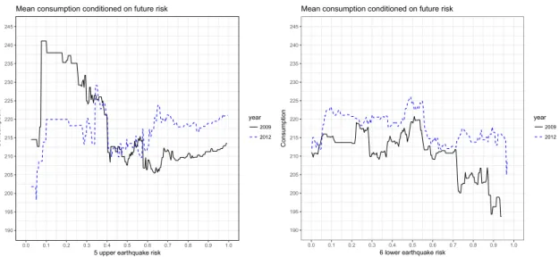
Figure 1: Average consumption conditional on the risk of being hit by a large-scale earthquake. The left-hand figure describes the local average consumption conditional on the probability that a household suffers an earthquake of a JMA seismic intensity larger than 6 lower in the next 30 years. The right-hand figure describes the local average consumption conditional on the probability that a household suffers an earthquake of a JMA seismic intensity larger than 5 upper in the next 30 years.
such models to reveal preference parameter changes using observational data.
We extend the literature by introducing heterogeneity into preference parameters. The heterogeneity may arise from future risks of a similar disaster faced by households. For example, Goebel, Krekel, Tiefenbach, and Ziebarth (2015) shows that risk averse-ness is differently affected depending on future risks represented by the geographic dis-tance between respondents’ residencies and the nearest nuclear power plant. Although types of future risks that introduce heterogeneity may be controversial, we believe fu-ture earthquake risks could be a possible source for heterogeneity in our set-up: we use Keio Household Panel Survey (KHPS) data and focus on the Great East Japan Earth-quake that occurred in March 2011. Figure 1 shows the mean consumption conditional on the probability of being hit by a future earthquake. These figures show that the change in consumption before and after the earthquake is heterogeneous across future earthquake risks. Households that face a lower earthquake risk decrease their
consump-tion, while those that face a higher risk increase their consumption on average. This finding suggests that the effects of earthquakes on the preference parameters may vary according to the future earthquake risks faced by households.
We find that the disaster affects households’ risk and time preference parameters. The observed effect is heterogeneous with respect to a household’s future risk of being hit by severe earthquakes. In particular, households facing a high risk of earthquakes become more risk averse compared with households facing a low risk of earthquakes. This result is consistent with German evidence reported by Goebel et al. (2015) and Bauer, Braun, and Kvasnicka (2017), that is, the Great East Japan Earthquake affected the risk attitudes of households facing the risk of a similar disaster in the future even if they did not directly experience the disaster themselves. Our result is also consistent with Ishino, Kamesaka, Murai, and Ogaki (2012) and Sekiya et al. (2012), who analyze the earthquake from a psychological perspective. Our simulation shows that the risk and time preference parameters estimated from data before the earthquake can severely under- or overestimate the consumption expenditure of households after the disaster.
These results are robust to measurement error in consumption (see, for example, Runkle, 1991 who confirms the existence of measurement errors in consumption data when testing the permanent income hypothesis). We employ D and GMM-LN estimators proposed by Alan, Attanasio, and Browning (2009) (see, also Ventura, 1994 and Chioda, 2004). For consistency, these estimators require strong assumptions such that the measurement errors in consumption are independent from the level of consumption and/or the distribution of measurement errors is known, which might be implausible to assume in some economic data (e.g., Bound & Krueger, 1991, Bound, Brown, Duncan, & Rodgers, 1994, and Chen, Hong, & Tamer, 2005). For example, the accuracy of the consumption measurement may depend on the level of consumption. Since a 10% measurement error at a high level of consumption is larger than that at a low level, households with higher expenses may have a greater measurement error than
those with lower expenses.
To check the robustness of these assumptions, we propose a new identification strat-egy for the preference parameters in life-cycle consumption models when consumption is contaminated by dependent measurement errors.2 It reveals the set of parameters char-acterized by moment inequalities evaluated with the observed consumption, to which the true parameters belong. The only assumption required in this study is the weak sta-tionarity of measurement errors. The confidence sets for parameters satisfying moment conditions, which can be inferred by existing methods, such as Chernozhukov, Hong, and Tamer (2007), can be used to test the underlying assumptions set for GMM-D and GMM-LN estimators.
The remaining paper is organized as follows. Section 2 explains the empirical back-ground of the study and Section 3 presents the economic model. We describe the analytical strategy based on the economic model and propose the test for the assump-tions on measurement errors in Section 4. The proof for the proposition is given in the Appendix. Sections 5 and 6 present the data and the empirical results, respectively. The conclusion and policy implications of the study are discussed in Section 7.
2
Empirical Background
2.1
The Great East Japan Earthquake and Related Studies
The Great East Japan Earthquake hit the eastern coast of Japan on March 11, 2011. The earthquake caused a tsunami, leading to 15, 800 deaths, 2, 500 missing persons, 6, 000 injuries, 450, 000 evacuations, and the Fukushima nuclear accident. The disaster
2In the recent approach by Gayle and Khorunzhina (2017), the author uses information on additional
time periods that comes from habit formation in preferences. Their independence assumption is mild in the sense that they only assume independence between the growth rates of consumption and measurement errors. Without habit formation, however, this approach fails to identify the time discount factor.
caused power outages and water shortages not only on the eastern coast of Japan, but also in the areas surrounding Tokyo. These events were repeatedly broadcast across Japan. Therefore, the Great East Japan Earthquake may have affected not only the households in disaster-hit areas, but also the entire population of Japan.
Researches adopting hypothetical questionnaires and experiments imply that the disaster changed Japanese households’ preference parameters. Sawada and Kuroishi (2016) investigated how risk and time preference parameters are differently affected by the level of housing damage. The authors conducted a field experiment after the disaster, and found that the disaster affected the present bias parameter negatively. Hanaoka et al. (2018) focus on the link between individuals’ hypothetically elicited risk aversion parameters and the seismic intensity of the earthquake experienced by them, finding that men who experience an earthquake of large seismic intensity become risk tolerant. Goebel et al. (2015) analyzed the risk and political attitudes of Germans by using a questionnaire, and found that the Great East Japan Earthquake and the sub-sequent disaster affected the risk attitudes of Germans. Ishino et al. (2012) and Sekiya et al. (2012) suggest that the psychological impact of the earthquake was not limited to individuals who physically experienced the disaster, showing that it also affected individuals facing future risks of similar large-scale disasters. This study contributes to the literature in accumulating empirical evidences obtained by observational data.
2.2
Future Earthquake Risk
This study estimates preference parameters in life-cycle consumption models by using the Euler equation (first order condition) as the moment restriction. We use observa-tional household panel data, and compare the estimates before and after the disaster at each future earthquake risks. Especially, we use the localized moment restrictions directly implied by the Euler equation and adopt the localized GMM-D and GMM-LN
estimators (see, Lewbel, 2007 for local GMM estimator). By localizing the moment conditions, we implicitly assume that households that have similar characteristics hold the same information and the same prediction about their future.
For the earthquake risk measures, we use the data on probabilistic earthquake haz-ards published by the Japan Seismic Hazard Information Station (JSHIS) together with the Geographic Information System of the University of Tokyo.3 We adopt two
prob-abilities: a location will be hit by an earthquake with a Japan Meteorological Agency (JMA) seismic intensity larger than 5 upper in the next 30 years (5 upper risk here-after) and a JMA seismic intensity larger than 6 lower in the next 30 years (6 lower risk hereafter).4
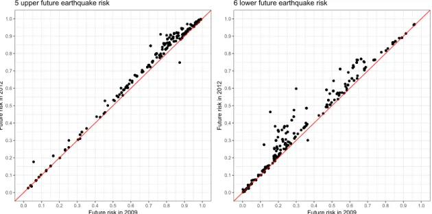
Figure 2 illustrates the geographical distribution of the future earthquake risk. Fig-ure 3 shows the relationship between the probabilistic seismic hazards of 2009 and 2012. Although the reported future risks faced by each household are not the same across these two years, the observed change in the future earthquake risk before (2009) and after (2012) the earthquake is small, indicating that the local moments capture almost the same households across these years. Comparing the parameter estimates in 2009 and 2012 at a specific future risk is possible; however, the interpretation of the results in this study is compared carefully, especially for those households whose 6 lower risk in 2009 lies between 0.2 and 0.8 and for those households whose 5 upper risk in 2009 lies between 0.5 and 0.9.
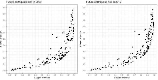
Figure 4 displays the positive correlation between the 5 upper and 6 lower earthquake risks. In particular, households facing a high 6 lower risk of around 0.9 also face a 5 upper risk of above 0.9, while those facing a low 5 upper risk of around 0.1 also face a
3http://newspat.csis.u-tokyo.ac.jp/geocode/.
4JMA seismic intensity is the measure of the seismic intensity at a particular location, which
ranges from 0 to 7. The value is mainly related to land acceleration caused by the earthquake. The detailed descriptions for seismic intensity are given by the Japan Meteorological Agency under http://www.jma.go.jp/jma/en/Activities/inttable.html. Although the seismic magnitude is used to measure the overall strength of an earthquake, JMA seismic intensity is an appropriate measure for local seismic intensity.
Figure 2: Geographical distribution of future earthquake risks. The right-hand figure describes the probability that a location suffers an earthquake of a JMA seismic intensity larger than 6 lower in the next 30 years. The left-hand figure describes the probability that a location suffers an earthquake of a JMA seismic intensity larger than 5 upper in the next 30 years.
0.0 0.1 0.2 0.3 0.4 0.5 0.6 0.7 0.8 0.9 1.0 0.0 0.1 0.2 0.3 0.4 0.5 0.6 0.7 0.8 0.9 1.0 Future risk in 2009 F ut ure ri sk in 2 01 2
5 upper future earthquake risk
0.0 0.1 0.2 0.3 0.4 0.5 0.6 0.7 0.8 0.9 1.0 0.0 0.1 0.2 0.3 0.4 0.5 0.6 0.7 0.8 0.9 1.0 Future risk in 2009 F ut ure ri sk in 2 01 2
6 lower future earthquake risk
Figure 3: Relationship between the future earthquake risks measured in 2009 and 2012. The left-hand figure shows the probability of suffering a JMA seismic intensity larger than 5 upper in the next 30 years. The right-hand figure shows the probability of suffering a larger than 6 lower earthquake.
0.0 0.1 0.2 0.3 0.4 0.5 0.6 0.7 0.8 0.9 1.0 0.0 0.1 0.2 0.3 0.4 0.5 0.6 0.7 0.8 0.9 1.0 5 upper intensity 6 lo w er in te nsi ty
Future earthquake risk in 2009
0.0 0.1 0.2 0.3 0.4 0.5 0.6 0.7 0.8 0.9 1.0 0.0 0.1 0.2 0.3 0.4 0.5 0.6 0.7 0.8 0.9 1.0 5 upper intensity 6 lo w er in te nsi ty
Future earthquake risk in 2012
Figure 4: Relationship between the 6 lower and 5 upper future earthquake risks.
low 6 lower risk of under 0.1.
2.3
Behavioral Changes through Preference Parameter
There are at least three channels through which natural disasters may affect households’ consumption behavior. They are budget constraint, belief, and preference parameter changes. A challenging issue to capture the preference parameter changes from observed households economic behavior is to exclude the first and second channels.
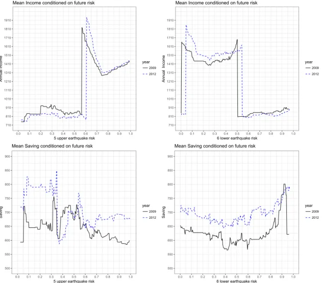
First, a natural disaster may damage properties and affect income or saving, which can alter budged constraints of households. To exclude this channel, we focus on house-holds whose properties are undamaged, and exclude househouse-holds whose income and sav-ing show substantive increase or decrease. Although excludsav-ing those households does not wipe out the channel completely, we do not find systematic relationships between the income growth and consumption or saving growth. Figure 5 shows expectation of income (upper figures) and saving (lower figures) conditional on the future earthquake risks. The expectation of income in 2012 is lower than that in 2009 for those whose
fu-710 810 910 1010 1110 1210 1310 1410 1510 1610 1710 1810 1910 0.0 0.1 0.2 0.3 0.4 0.5 0.6 0.7 0.8 0.9 1.0
5 upper earthquake risk
An nu al In co me year 2009 2012
Mean Income conditioned on future risk
710 810 910 1010 1110 1210 1310 1410 1510 1610 1710 1810 1910 0.0 0.1 0.2 0.3 0.4 0.5 0.6 0.7 0.8 0.9 1.0
6 lower earthquake risk
An nu al I nco me year 2009 2012
Mean Income conditioned on future risk
500 550 600 650 700 750 800 850 900 0.0 0.1 0.2 0.3 0.4 0.5 0.6 0.7 0.8 0.9 1.0
5 upper earthquake risk
Sa
vi
ng year2009
2012
Mean Saving conditioned on future risk
500 550 600 650 700 750 800 850 900 0.0 0.1 0.2 0.3 0.4 0.5 0.6 0.7 0.8 0.9 1.0
6 lower earthquake risk
Sa
vi
ng year2009
2012
Mean Saving conditioned on future risk
Figure 5: Average income and saving conditional on the risk of being hit by a large-scale earthquake. The right-hand figure describes the local average income (upper figure) and saving (lower figure) conditional on the probability that a household suffers an earthquake of a JMA seismic intensity larger than 6 lower in the next 30 years. The left-hand figure describes the local average income (upper figure) and saving (lower figure) conditional on the probability that a household suffers an earthquake of a JMA seismic intensity larger than 5 upper in the next 30 years.
ture risks are high (6 lower risk above 0.6). For these households, however, consumption in 2012 is higher than that in 2009, as shown in Figure 1. In the same manner, income for those whose future risks are low (5 upper risk under 0.5) and high (6 lower risk above 0.6) decreases, while their saving increases. These findings imply that economic behavior of these households changes during this period, which may come from belief updates or preference parameter changes.
Second, belief5 about the future states may be updated by experiencing natural
disasters, which changes households’ behavior. Distinguishing preference parameter changes from belief update by using observational data requires an assumption in which households have homogenous beliefs about future states. Under this assump-tion, updated belief is reflected in empirical distributions of economic variables after the disaster, implying that the preference parameter changes observed by comparing the estimates before and after the disaster are distinguished from belief updates. Then, the homogenous belief assumption is crucial to identify preference parameter changes from observational data. This assumption is also a part of complete market assumption required for the estimation of parameters using Euler equations when one uses short periods of data (see, Chamberlain, 1984 and Hayashi, 1985 ).6
An approach to moderate this limitation of a homogenous belief assumption involves the introduction of heterogeneous preference parameters, which reduces the degree of homogeneity. This study introduces heterogeneous preference parameters depending on the future earthquake risk faced by households. Then, only the households that face similar future risk are required to have homogenous beliefs about future states.
5Formally, we define belief as the conditional distribution of the future state of the world. Suppose,
for simplicity, that the future state of the world considered at time t is discrete and finite, which we denote as st∈ {1, 2, . . . , S}. Then, one’s belief is that the conditional probability of the future state is
P (st|It), where information set It includes all the information about the economic variables that are
consequences of the realized state at time t. A belief update caused by an event indicates that the belief of a future state after the event is different from that before the event.
3
Economic Model
We specify households’ behavior using the life-cycle consumption models. We assume that a household chooses the intertemporal allocation of consumption and investment that maximizes its expected utility is not subject to liquidity constraints, and has an additive budget over time. Further, utility is intertemporally additive, that is, it has no habit formation specification.
At time t, household i chooses (non-durable) current and future consumption Ci,t
and investment plan Qi,t =
∑J
j=1Ai,j,t—which is a summation of J assets Ai,j,t—to
maximize the expected utility function, given information set It available at time t.
Households’ expected utility maximization problem is
max E [ ∞ ∑ t=0 βtU (Ci,t, xi, γ) Ii,t ] ,
s.t. Qi,t+1 ≤ Qi,t(1 + Ri,t) + Li,t− Ci,t (1)
where 0 < β < 1 is the discount factor, and U (·) represents a strictly concave utility function with the household fixed effect xi and utility curvature parameter 0 < γ < ∞.
Specifically, we assume the utility function to be the constant relative risk aversion (CRRA) type: U (Ci,t, xi, γ) = (1− γ)−1(C
1−γ
i,t − 1) exp(xi). Since γ represents the
Arrow–Pratt measure of relative risk aversion under CRRA utility, we call it the risk parameter.7 The household’s returns R
i,t at time t consist of the weighted average
returns of its assets, where the weight is quantity. Li,t is labor income at time t.
The first-order condition of the maximization problem is
E{β(1 + Ri,t+1) (Ci,t+1/Ci,t)−γ − 1 Ii,t
}
= 0, (i = 1, . . . , N ). (2)
7We assume that CRRA-type utility may be too restrictive, since all households are assumed to have
identical preference parameters. We moderate this assumption by considering the varying coefficients model in which we allow the preference parameters to differ across households’ characteristics.
The information set at time t consists of all the variables known by the households, that is, Ii,t = {Ri,s, Ci,s, Zi,s, νi,s}ts=t0, where Zs is a vector of the variables observable
by the researchers, νi,s represents the variables observable by the households but not
the researchers, and t0 is the initial period.
4
Estimation Strategy
To introduce the heterogeneous preference parameters, we localize the Euler equation (2). The utility maximization problem conditioned by Ii,t and the localizing variables,
say, Wi, yield the Euler equation: E[β(w)(1 + Ri,t+1)(Ci,t+1/Ci,t)−γ(w) − 1|Ii,t, Wi,t =
w] = 0, where β and γ are now functions of Wi,t, which directly implies
E{[β(w)(1 + Ri,t+1)(Ci,t+1/Ci,t)−γ(w)− 1]|Zi,t, Wi,t = w} = 0, (3)
for Zi,t ∈ Ii,t. Note that equation (3) is directly implied by the first-order condition (2)
as long as the localizing variable Wi is in the household’s information set. Otherwise,
the population of interest should be those with a localizing variable equal to w.
We use equation (3) as the moment conditions, and estimate β(w) and γ(w) by employing the localized version of the GMM-D and GMM-LN estimators, which are measurement error-robust estimators proposed by Alan et al. (2009). The GMM-D estimator assumes measurement errors to be stationary and independent of all compo-nents in the information set, including the lagged value of measurement errors, con-sumption, interest rate, and instruments. In addition to stationarity and independence, the GMM-LN estimator requires the measurement error to follow a normal distribution with the same variance across households and includes the variance as an additional parameter to be estimated.
4.1
Moment Inequality Approach
To test the validity of assumptions set on the measurement errors in the GMM-D and GMM-LN estimators, we propose a novel moment inequality approach to obtain a confi-dence set that requires milder assumptions on the measurement errors. Conficonfi-dence sets are useful because when the GMM-D and GMM-LN estimates lie outside the confidence sets, we can conclude that the assumptions set on measurement errors are unreliable.
Let true consumption Ci,t be observed with the multiplicative error ηi,t such that
the observed consumption is given by Ci,tobs = Ci,tηi,t. The multiplicative measurement
error of consumption is standard in the literature on life-cycle consumption models. For notational simplicity, we denote the measurement error of log consumption by
ϵi,t ≡ log Ci,tobs− log Ci,t = log ηi,t.
Assumption 1 (Measurement error). For each household with the same future risks,
ϵt is weakly stationary for two time periods, namely, before and after the disaster.
Assumption 1 is the only assumption set on measurement errors to derive confidence sets. It does not require any independence between the errors and other variables. For example, it allows measurement errors to depend on the level of consumption, demographic characteristics, and even unobservable household characteristics. The stationarity assumption also allows serial correlation of measurement errors that occurs if the household tends to over- or under-report the level of consumption. In existing methods, serial correlation of measurement errors is not allowed except in Gayle and Khorunzhina (2017).
Under Assumption 1, we can transform (3) into moment inequalities expressed in terms of the observed consumption
E
{
log β(w)(1 + Ri,t+1)− log E[g(Zi,t)|Wi,t = w]− γ(w) log
( Ci,t+1obs Cobs i,t ) + log g(Zi,t) Wi,t = w } ≤ 0, (4)
for any measurable transition function g(·). The derivation of (4) is shown in the proof of Proposition 1.8
4.2
Identification
We show that the true parameters satisfying the baseline moment conditions (3), if they exist, belong to an informative parameter set consistent with the moment inequalities defined in (4). Let θ(w) ={β(w), γ(w)}. For notational simplicity, we define ρi,t(θ) =
β(w)(1 + Ri,t+1) (Ci,t+1/Ci,t)−γ(w) and ρobsi,t (θ) = β(w)(1 + Ri,t+1)
(
Cobs
i,t+1/Ci,tobs
)−γ(w) . Then, our baseline moment restriction (3) is E{ρi,t[θ(w)]−1|Zi,t, Wi,t = w} = 0, and the
moment inequality (4) is E{log ρobs
i,t [θ(w)]− log E[g(Zi,t)|Wi,t = w] + log g(Zi,t)|Wi,t =
w} ≤ 0. Let the true preference parameter vector be θ0(w)≡ {β0(w), γ0(w)}, that is,
θ0(w) = {θ(w) : E{ρi,t[θ(w)]− 1|Zi,t, Wi,t = w} = 0}.
For the identification, we need the following assumptions along with Assumption 1.
Assumption 2 (Completeness). E{ρi,t[θ(w)]− 1|Zi,tWi,t = w} = 0 implies ρi,t[θ(w)]−
1 = 0 a.s. for some t.
Assumption 3 (Rank). E[(1, log(Ci,t+1/Ci,t))′(1, log(Ci,t+1/Ci,t))] has full rank for all
t.
We follow existing works, such as Gayle and Khorunzhina (2017), for the complete-ness assumption to ensure comparability. The completecomplete-ness restriction in Assumption 2 is satisfied, for example, when the joint distribution of{Ci,t, Ci,t+1, Ri,t+1} belongs to
exponential families. Other sufficient conditions can be found, for example, in Hu and Shiu (2017).
8Assumption 1 does not allow measurement errors to have a time trend that occurs when the
experiences of respondents mitigate measurement errors over time. For identification of parameters and deriving inequalities (4), Assumption 1 can be replaced with one that arrows time trend in mea-surement errors. That is, inequality (4) can be derived under a milder assumption that arrows time trend. The assumption that arrows time trend restricts the expectation of (the inverse of) the growth of the measurement errors. See, Iwasawa and Nakanishi (2018), for the assumption and following identification.
The rank condition in Assumption 3 requires the consumption growth to vary across households. The rank condition is violated, for example, when all households have equivalent consumption growth, meaning that the second moment of the consumption growth is equal to the square of its first moment.
Proposition 1. Suppose Assumptions 1, 2, and 3 hold. Then, θ0(w) is identified if
E{ρi,t[θ(w)]− 1|Zi,tWi,t = w} = 0. Moreover, θ0(w) belongs to the set of parameters
satisfying (4).
The first statement in Proposition 1 about the identification of the preference param-eters is not new. For example, Gayle and Khorunzhina (2017) shows the identification of the parameters in the Euler equation under habit forming utility by assuming the completeness and rank restrictions. We show the identification results to clarify the true parameter in which we are interested.
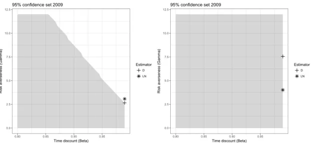
The second part of Proposition 1 states that the true parameter vector satisfying the Euler equation is consistent with the moment inequality (4). The results of Proposition 1 are useful in at least two senses. First, the parameter set satisfying these inequalities pins down the potential parameter space that contains the true parameters, which is obtained by using the information provided by the data and weak assumption on measurement errors. The parameter space may help to determine the initial parameter values for optimization. Second, the moment inequality approach can be used as a sensitivity analysis of other approaches such as GMM-D and GMM-LN estimators. The assumptions on measurement errors required by these estimators are rejected when these estimates lie outside the parameter set (see, Figure 6 for an example of confidence set).
0.0 2.5 5.0 7.5 10.0 12.5 0.80 0.85 0.90 0.95
Time discount (Beta)
R isk ave rse ne ss (G amma ) Estimator D LN 95% confidence set 2009 0.0 2.5 5.0 7.5 10.0 12.5 0.80 0.85 0.90 0.95
Time discount (Beta)
R isk ave rse ne ss (G amma ) Estimator D LN 95% confidence set 2009
Figure 6: 95% confidence sets and estimated parameter values. The 95% confidence sets for time discount factors β (vertical line) and risk averseness parameters γ (horizontal line) are shadowed.
4.3
Inference
We adopt the method developed by Chernozhukov et al. (2007) to derive the 95% confidence set for the preference parameters γ and β that satisfy the moment inequality (4).
Let m(θ) be the vector of the moment restrictions and ΘI denote the parameter
values that satisfy the moment restrictions, that is, ΘI = {θ : m(θ) ≤ 0}. In our case,
the moment restriction is (4). The confidence region is denoted as Cn(c) ≡ {θ ∈ Θ :
nQn(θ) ≤ c}, where Qn(θ)≡ ∥ max[mn(θ), 0]∥2for empirical moment mn(·) of m(·) and
c is a consistent estimate of the α-quantile of supθ∈θInQn(θ). We follow the subsampling
method of Chernozhukov et al. (2007) to obtain c, and calculate it by using Bn = 100
draws of subsamples of size b = n/2.9 We begin with a starting value ˆc
0 of c.10 We
9Since there is no general theory to choose the size of the subsample, we follow Gayle and
Khorun-zhina (2017). Another example is n/4, which is used by Ciliberto and Tamer (2009).
10We randomly choose 100 sets of the initial parameter values, which we denote as ¯Θ. The
start-ing value ˆc0 is chosen to be infθ∈¯θnQn(θ). Attanasio and Weber (2010) reviewed the literature on
consumption-based estimates of the relative risk aversion parameter to show estimates that range be-tween 1 and 3. Less empirical evidence has been accumulated for the discount factor, since it is not
compute supθ∈Cn(c0)bQj,b(θ) for each subsample j = 1, . . . , Bn, where Qj,b(θ) denotes
the criterion function evaluated by using the jth subsample. Then, we calculate ˆc1 as
the α-quantile of these quantities. Similarly, we calculate ˆc2 and ˆc3. The critical value
is set to be c = min(ˆc1, ˆc2, ˆc3).
5
Data
5.1
Data Sources
Five data sources are used in this study. The first is KHPS data, which include house-hold behavior and information on househouse-holds’ assets. The second data source is the average interest rates of deposits posted at financial institutions by type of deposit from 2007 to 2015. These data are available from the website of the Bank of Japan. The third data source is the average price and yield of securities, which is published by the Tokyo Stock Exchange. The fourth is the probabilistic seismic hazard data published by the JSHIS. The fifth data source is the observed seismic intensity caused by the Great East Japan Earthquake.
The KHPS is a panel survey of household behavior and social attitudes that has been conducted since 2004. The survey respondents of the KHPS are selected by two-stage stratified sampling. The number of survey respondents was 4, 005 in 2004. The KHPS added new cohorts in 2007 and 2012 (1, 419 respondents in 2007 and 1, 012 respondents in 2012). The survey subjects of the KHPS are men and women aged 20 to 69 years. The KHPS data consist of information on households’ consumption, saving, security, debt, socio-demographic characteristics, and city of residence. The survey is conducted in January, and respondents are asked to report consumption details for January and
identified by using the conventional log-linear method. According to Alan et al., 2009, who provide a rare example, β is around 0.95, and it is not plausible for β to be close to zero. Therefore, each θ∈ ¯Θ is randomly chosen from [0.5, 1] for β and [1, 3] for γ.
their current saving, security, debt, and socio-demographic characteristics.
5.2
Data Used in the Study
The findings of Sekiya et al. (2012), Ishino et al. (2012), Goebel et al. (2015), and Bauer et al. (2017) imply that the Great East Japan Earthquake affected not only those individuals who experienced the earthquake, tsunami, and nuclear accident, but also those who did not. To analyze the indirect effect of the disaster, we do not limit our focus to households in eastern Japan. Our data thus covers households across Japan.
We use the sample of nuclear families with at least one child and whose head is of working age during the sample periods, from 2007 to 2015, namely, a household head no older than 51 years and no younger than 16 years in 2007. To apply our theoretical model, we focus on households that satisfy the following characteristics. First, following Attanasio and Weber (1995) and Vissing-Jørgensen (2002), we drop observations for which the observed income and consumption growth ratios in 2009 and 2012 are less than 0.2 or above five (73 households) to exclude obvious reporting and coding errors. Second, following Alan et al. (2009), we exclude households that have no saving during the sampling periods (186 households) to exclude any households that may be liquidity-constrained in the sample periods. Third, we remove households whose properties were substantially damaged by the earthquake (one household).11
While the exclusion of households with an abrupt consumption growth ratio is standard in the literature, such exclusion according to income and properties may be non-standard. Under the permanent income or risk-sharing hypotheses, unexpected income shocks do not affect household consumption. However, empirical studies using Japanese data show skeptical evidence of the risk-sharing hypothesis, especially when households are liquidity constrained. For example, Kohara, Ohtake, and Saito (2006), Ichimura, Sawada, and Shimizutani (2008), and Sawada and Shimizutani (2008) provide
empirical evidence using Japanese data, while Ogaki and Zhang (2001) and Zhang and Ogaki (2004) tested the risk-sharing and permanent income hypotheses. Therefore, we concentrate on those households whose economic environment was not substantially affected by the earthquake and that were not liquidity-constrained.
We remove households that did not submit the questionnaire at least once from 2007 to 2015. The original sample size is 2, 864 for 2007, 3, 691 for 2008, 3, 422 for 2009, 3, 207 for 2010, 3, 030 for 2011, 2, 865 for 2012, 3, 568 for 2013, 3, 305 for 2014, and 3, 124 for 2015. The number of households that submitted all questionnaires in the period is 2, 658. The number of nuclear family households that satisfy the conditions stated above is 278. The first and second panels of Table 1 present the summary statistics of the household characteristics in 2009 and 2012, respectively.
5.3
Consumption
For the composition of consumption, we follow Hall (1978) and the empirical evidence presented by Khvostova, Larin, and Novak (2016) and Gayle and Khorunzhina (2017). They includes non-durable consumption and services, which is a standard definition used in time-separable utility models (e.g., Attanasio & Weber, 1995, Vissing-Jørgensen, 2002, and Alan, 2012). Specifically, consumption is the sum of expenditure on food con-sumed at home and away from home, lighting, heating, water, fuel, public transport, and communication services. All of them are available in KHPS data. Data on con-sumption are deflated by using the consumer price index at the prefecture level.12
In contrast to a large number of studies that use the Panel Study of Income and Dynamics (PSID), such as Shapiro (1984), Runkle (1991), Alan et al. (2009), Alan and Browning (2010), and Alan, Browning, and Ejrnæs (2018), we do not focus on food consumption. A notable reason is that the utility function we adopt does not have a habit formation specification, meaning that current consumption affects utility only in
Table 1: Summary statistics of the data used in the study
mean median std.dev min max 2009
Age of the household head 42.04 5.73 42 29 52
Number of children 2.01 0.69 2 1 5
Saving 606.49 712.37 400 20 5252
Annual income 816.24 397.67 736 179 4065
Future risk 6 lower 0.35 0.26 0.25 0.00 0.96 Future risk 5 upper 0.74 0.81 0.25 0.03 0.99 2012
Age of the household head 45.04 5.73 45 32 55
Number of children 2.03 0.71 2 1 5
Saving 694.96 832.19 460 5 6940
Annual income 822.47 330.52 750 180 1900
Future risk 6 lower 0.39 0.36 0.25 0.00 0.97 Future risk 5 upper 0.76 0.86 0.25 0.03 1.00 Consumption rate C2010/C2009 1.025 0.293 0.980 0.481 2.767 C2013/C2012 1.054 0.297 1.019 0.374 3.000 Return (%) R2009 -0.215 0.193 0.908 -4.646 0.243 R2010 -1.359 0.065 3.169 -17.242 0.088 R2012 3.202 0.026 7.303 0.026 40.062 R2013 0.142 0.026 0.268 0.026 1.494
Note: Annual income is pre-tax annual household income of the previous year. Saving
indicates the amount of household total saving at the moment of the response. Both are given in 10 thousand Japanese yen.
the current period. Gayle and Khorunzhina (2017) used the PSID to show that habit formation is an important determinant of food consumption patterns. Alternatively, Khvostova et al. (2016) used Russian panel data that contain rich information on non-durable consumption other than food; they found that habit formation is not significant. Therefore, we follow the results of Khvostova et al. (2016) to compose consumption.13
13A growing body of the literature has offered empirical evidence of habit formation for consumption.
The existence of habit formation is inconclusive, however, and may depend on the types of consumption and data sets used. For example, Dynan (2000) found no habit formation on foods by using the PSID, while Carrasco, Labeaga, and J David (2005) and Browning and Collado (2007) show habit
The third panel of Table 1 shows the descriptive statistics for the growth rates of consumption. The mean consumption rates are stable over time, showing that con-sumption is smoothed. The growth rates of concon-sumption are slightly higher after the earthquake leading to the conjecture according to which households may become risk tolerant and/or have a lower discount factor.
5.4
Household-Specific Returns
Household-specific returns Ri,t are calculated by using the average interest rates of
deposits data, average price and yield data, and households’ saving and asset amounts included in the KHPS data.
The average interest rates of deposits data show the average interest rate of the Bank of Japan’s clients.14 We calculate households’ interest rates for deposits by using
the average interest rates of deposits data, which include the average interest rates for three deposit amounts: less than 300, 000 JPY, from 300, 000 to 1, 000, 000 JPY, and more than 1, 000, 000 JPY. Households’ interest rates for deposits are calculated as
ri,saving,t=1{savingi,t < 300, 000 JPY}r(300, 000, t)
+1{300, 000 JPY ≤ savingi,t < 1, 000, 000 JPY}r(1, 000, 000, t)
+1{1, 000, 000 JPY ≤ savingi,t}r(1, 000, 000+, t), (5)
formation for food, but a non-significant habit pattern in transport by using Spanish panel data, Leth-Petersen (2007) shows habit formation for gas for heating by using Danish panel data, and Guariglia and Rossi (2002) show habit patterns in food consumption by using British panel data. However, the empirical results of Khvostova et al. (2016) and Gayle and Khorunzhina (2017) are obtained by adopting measurement error-robust methods, which are not used in other works. They are also the earliest studies to use the exact Euler equation non-linear GMM method wherein no distributional assumption on the measurement errors is set. Therefore, we follow their results.
14These include city banks, regional banks, the second association of regional banks, trust banks,
credit unions, and the Shoko Chukin Bank. City banks include Mizuho Bank, Bank of Tokyo-Mitsubishi UFJ, Sumitomo Mitsui Banking Corporation, Resona Bank, and Saitama Resona Bank. Regional banks are member banks of the Regional Banks Association of Japan. Trust banks are those that, in addition to banking businesses, operate trust businesses based on the Act on Provision, and so on, of Trust Business by Financial Institutions and are not categorized as city or trust banks.
where r(300, 000, t) is the average interest rate for a deposit for which the amount is less than 300, 000 JPY when time is equal to t; r(1, 000, 000, t) is the average interest rate for a deposit for which the amount is more than 300, 000, but less than 1, 000, 000 JPY when time is equal to t; and r(1, 000, 000+, t) is the average interest rate for a deposit for which the amount is less than 1, 000, 000 JPY when time is equal to t.
The average price and yield data published by the Tokyo Stock Exchange consist of average yield for securities traded in the first and second sections of the Exchange. In this study, we use the annual average price and yield of securities, say, ri,security,t,
which are the weighted average of the monthly average price and yield as the return to securities.
Then, household-specific return Ri is calculated as
Ri,t = ri,saving,t Ai,saving,t Ai,saving,t+ Ai,security,t + ri,security,t Ai,security,t Ai,saving,t+ Ai,security,t , (6)
where Ai,saving,tis household i’s saving at time t and Ai,security,tis household i’s securities
at time t. The fourth panel of Table 1 shows the descriptive statistics of household-specific returns.
6
Results
Following Alan et al. (2009) and Gayle and Khorunzhina (2017), the set of instruments include the number of children, lagged household-specific returns, and a constant; the future earthquake risks (5 upper and 6 lower) are also included for the localization.
The bandwidths for the non-parametric kernel estimation of the localized models are obtained by cross-validation. First, we estimate the parameters for a specific value of the localizing parameter W = w, which we denote as ˆθ1(w), by using the bandwidth
(CUGMM) to obtain the estimates, as suggested by Hansen, Heaton, and Yaron (1996). Second, ˆθ1(w) is plugged into the local GMM objective function so that it can be seen
as a function of the bandwidths. We find the bandwidths that minimize the objective function, which we denote as ˆh1. The final estimation results are then estimated by
using ˆh1 instead of the rule of thumb bandwidth in the first step.
We adopt the future earthquake risk (6 lower and 5 upper) variables as the localizing variables and estimate the parameters at equally spaced 99 localizing points in the [0.01, 0.99] interval.15 Figures 7, 8, 9, and 10 present the estimation results for the 6
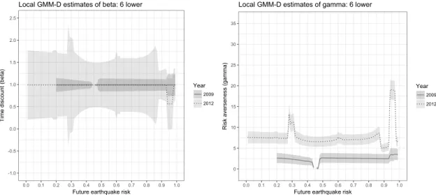
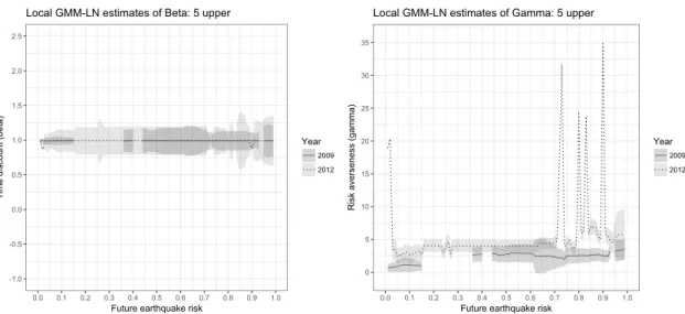
lower future risk of the GMM-D and GMM-LN estimators and 5 upper future risk of the GMM-D and GMM-LN estimators, respectively. In these figures, the results for each localizing point are displayed only when the estimates both before and after the earthquake belong to the 95% confidence set derived by moment inequalities (4). In other words, we show the results of the localizing points in which our moment inequality does not reject the additional distributional assumptions imposed on the GMM-D and GMM-LN estimators.
6.1
Results for 6 Lower Future Risk
The GMM-D estimates of the discount factor parameter β in the left panel of Figure 7 suggest that the discount factors of most households in 2009 are close to one and do not change in 2012. The only exception is households whose future earthquake risks lie between 0.94 and 0.97. The discount factors of these households are lower after the earthquake. However, the 95% confidence intervals of the estimated discount factor overlap, which suggests that the change in parameters might not be statistically signif-icant. Overall, we can conclude that no subpopulation shows any significant discount factor changes.
15As shown in descriptive statistics of Table 1, we have no observations that face a future earthquake
-1.0 -0.5 0.0 0.5 1.0 1.5 2.0 2.5 0.0 0.1 0.2 0.3 0.4 0.5 0.6 0.7 0.8 0.9 1.0
Future earthquake risk
T ime d isco un t (b et a) Year 2009 2012
Local GMM-D estimates of beta: 6 lower
0 5 10 15 20 25 30 35 0.0 0.1 0.2 0.3 0.4 0.5 0.6 0.7 0.8 0.9 1.0
Future earthquake risk
R isk ave rse ne ss (g amma ) Year 2009 2012
Local GMM-D estimates of gamma: 6 lower
Figure 7: The local GMM-D estimates and 95% confidence intervals for the 6 lower future risk. Only the estimation results within the 95% confidence sets derived by the moment inequalities are displayed.
-1.0 -0.5 0.0 0.5 1.0 1.5 2.0 2.5 0.0 0.1 0.2 0.3 0.4 0.5 0.6 0.7 0.8 0.9 1.0
Future earthquake risk
T ime d isco un t (b et a) Year 2009 2012
Local GMM-LN estimates of beta: 6 lower
0 5 10 15 20 25 30 35 40 0.0 0.1 0.2 0.3 0.4 0.5 0.6 0.7 0.8 0.9 1.0
Future earthquake risk
R isk ave rse ne ss (g amma ) Year 2009 2012
Local GMM-LN estimates of gamma: 6 lower
Figure 8: The local GMM-LN estimates and 95% confidence intervals for the 6 lower future risk. Only the estimation results within the 95% confidence sets derived by the moment inequalities are displayed.
-1.0 -0.5 0.0 0.5 1.0 1.5 2.0 2.5 0.0 0.1 0.2 0.3 0.4 0.5 0.6 0.7 0.8 0.9 1.0
Future earthquake risk
T ime d isco un t (b et a) Year 2009 2012
Local GMM-D estimates of beta: 5 upper
0 5 10 15 20 25 30 35 0.0 0.1 0.2 0.3 0.4 0.5 0.6 0.7 0.8 0.9 1.0
Future earthquake risk
R isk ave rse ne ss (g amma ) Year 2009 2012
Local GMM-D estimates of gamma: 5 upper
Figure 9: The local GMM-D estimates and 95% confidence intervals for the 5 upper future risk. Only the estimation results within the 95% confidence sets derived by the moment inequalities are displayed.
-1.0 -0.5 0.0 0.5 1.0 1.5 2.0 2.5 0.0 0.1 0.2 0.3 0.4 0.5 0.6 0.7 0.8 0.9 1.0
Future earthquake risk
T ime d isco un t (b et a) Year 2009 2012
Local GMM-LN estimates of Beta: 5 upper
0 5 10 15 20 25 30 35 0.0 0.1 0.2 0.3 0.4 0.5 0.6 0.7 0.8 0.9 1.0
Future earthquake risk
R isk ave rse ne ss (g amma ) Year 2009 2012
Local GMM-LN estimates of Gamma: 5 upper
Figure 10: The local GMM-LN estimates and 95% confidence intervals for the 5 upper future risk. Only the estimation results within the 95% confidence sets derived by the moment inequalities are displayed.
The GMM-D estimates of the risk aversion parameters in the right panel of Fig-ure 7 suggest that most households whose futFig-ure earthquake risk is above 0.2 become risk averse after the earthquake. Figure 7 shows that the 95% confidence intervals in 2009 and 2012 do not overlap for those households. In particular, in 2012, households whose earthquake risk was between 0.94 and 0.97 have high ˆγ values compared with
households whose risk is outside this interval. Close inspection reveals that the munici-palities in which the corresponding households live are located along the Pacific Ocean in Aichi and Shizuoka prefectures. In particular, these municipalities face high risks of subsequent disasters, such as tsunamis, so their government offices publish hazard maps for future disasters to inform and alert their residents. A similar tendency of the risk aversion parameter changes is also exhibited by households with a future risk between 0.28 and 0.31. However, as shown in Figure 3, some households with a future risk in 2012 lying between 0.28 and 0.31 experience future risk shifts, indicating that the preference parameter changes for those households may be induced not only by the disaster, but also by the risk shifts. Overall, the results suggest that earthquakes make most households risk averse. The effect is heterogeneous and households may become more risk averse after a disaster if they live in places at risk of a future natural disaster that may bring about severe damage.
Figure 8 presents the estimation results of LN. The estimated value of GMM-LN is similar to that of GMM-D. There are few differences in the discount factors before and after the earthquake (see the left panel of Figure 8). The risk aversion parameter in the right panel of Figure 8 illustrates that households whose future risk lies above 0.97 become risk averse. Although the change is not as drastic as the GMM-D results, it is significant. Some households with a future risk below 0.8 also become risk averse. However, since households with future risks between 0.2 and 0.8 experience future risk shifts, these parameter changes may not only be induced by the earthquake. Thus, the GMM-LN results also suggest that households become more risk averse after a disaster
if they live in places at a high risk of future natural disasters.
6.2
Results for 5 Upper Future Risk
Figures 9 and 10 present the estimation results of GMM-D and GMM-LN, respectively, when the 5 upper future risk is used as the localizing variable. The results for the discount factor (the left panel of Figures 9 and 10) show that there are few differences in the discount factors before and after the earthquake.
The GMM-D estimates of the risk aversion parameters in the right panel of Figure 9 suggest that households that face 5 upper earthquake risks lying above 0.97 become significantly risk averse after the disaster. The GMM-LN estimates in the right panel of Figure 10 also illustrate that these households become risk averse. However, the 95% confidence intervals overlap, which suggests that the change in parameters might not be statistically significant for the latter estimates. This finding is consistent with the results obtained from the 6 lower earthquake risk, because the 6 lower risk of these households is distributed above 0.60 (see, Figure 4) and the risk averseness changes captured by the GMM-LN estimators are less than those captured by the GMM-D estimators. Since households with future risks between 0.5 and 0.9 experience future risk shifts, the parameter changes captured in this interval may not only be induced by the earthquake.
Interesting results are obtained by using 5 upper risks as the localizing variable when we focus on households that face future risks between 0.03 and 0.15 (see the right panel of Figure 10). Although these households become risk averse after an earthquake, the parameter change might not be statistically significant for most. Indeed, significant parameter changes are reported only for households with 5 upper risks of 0.03, 0.04, and 0.14. The municipalities in which the corresponding households exist are located in Ishikawa, Toyama, Fukuoka, Kagoshima, and the inland of Fukushima, which do not
face the Pacific Ocean. Half of these municipalities do not even face the ocean, indicat-ing that they are not exposed to disasters such as tsunamis. Overall, the results from the 5 upper localization suggest that an earthquake does not affect the risk averseness of households that live in places at a low risk of future natural disasters.
6.3
Consumption Prediction
We next compare actual consumption with predicted consumption for each point of future earthquake risks. Actual consumption is the observed households’ non-durable consumption in 2013. To predict the non-durable consumption of each household, we fit the observed household-specific return in 2012 as a proxy for the return in 2013, non-durable consumption in 2012, and the estimated preference parameters before and after the disaster to the Euler equation.
Figure 11 illustrates the absolute mean difference in the consumption forecast errors in 10, 000 Japanese yen. That is, this figure shows the absolute mean of the consumption forecast errors based on the before-disaster parameter estimates minus that based on the after-disaster parameter estimates (updated preferences hereafter). The positive values in the figure show the smaller forecasts errors in forecasts based on the updated preferences, thus favoring the preference parameter estimates after the disaster to make an accurate prediction.
Overall, the updated preferences make fewer forecasts errors. In particular, the two left panels of Figure 11 show the preference for the updated preferences of households with 5 upper future earthquake risks below 0.2. According to our estimation results, these households become risk averse after the disaster. Although the risk preference changes may be non-significant for most of these households, as shown in Figure 10, the difference improves the consumption prediction slightly.
-6 -5 -4 -3 -2 -1 0 1 2 3 4 5 6 (0,0.1] (0.1,0.2](0.2,0.3](0.3,0.4](0.4,0.5](0.5,0.6](0.6,0.7](0.7,0.8](0.8,0.9] (0.9,1]
Future earthquake risk
C on su mp tio n Ab so lu te me an d iff ere nce (2 00 9 - 20 12
) Local GMM-D estimates: 5 upper
-6 -5 -4 -3 -2 -1 0 1 2 3 4 5 6 (0,0.1] (0.1,0.2](0.2,0.3](0.3,0.4](0.4,0.5](0.5,0.6](0.6,0.7](0.7,0.8](0.8,0.9] (0.9,1]
Future earthquake risk
C on su mp tio n Ab so lu te me an d iff ere nce (2 00 9 - 20 12
) Local GMM-D estimates: 6 Lower
-6 -5 -4 -3 -2 -1 0 1 2 3 4 5 6 (0,0.1] (0.1,0.2](0.2,0.3](0.3,0.4](0.4,0.5](0.5,0.6](0.6,0.7](0.7,0.8](0.8,0.9] (0.9,1]
Future earthquake risk
C on su mp tio n Ab so lu te me an d iff ere nce (2 00 9 - 20 12
) Local GMM-LN estimates: 5 upper
-6 -5 -4 -3 -2 -1 0 1 2 3 4 5 6 (0,0.1] (0.1,0.2](0.2,0.3](0.3,0.4](0.4,0.5](0.5,0.6](0.6,0.7](0.7,0.8](0.8,0.9] (0.9,1]
Future earthquake risk
C on su mp tio n Ab so lu te me an d iff ere nce (2 00 9 - 20 12
) Local GMM-LN estimates: 6 Lower
Figure 11: Absolute mean difference in the consumption forecast errors. The posi-tive values show the preference for a consumption forecast based on the after-disaster parameter estimates.
190 195 200 205 210 215 220 225 230 0.0 0.1 0.2 0.3 0.4 0.5 0.6 0.7 0.8 0.9 1.0
Future Earthquake Risk 5 Upper
C on su mp tio n Type Forecast True Local GMM-D Prediction 190 195 200 205 210 215 220 225 230 0.0 0.1 0.2 0.3 0.4 0.5 0.6 0.7 0.8 0.9 1.0
Future Earthquake Risk 6 Lower
C on su mp tio n Type Forecast True Local GMM-D Prediction 190 195 200 205 210 215 220 225 230 0.0 0.1 0.2 0.3 0.4 0.5 0.6 0.7 0.8 0.9 1.0
Future Earthquake Risk 5 Upper
C on su mp tio n Type Forecast True Local GMM-LN Prediction 190 195 200 205 210 215 220 225 230 0.0 0.1 0.2 0.3 0.4 0.5 0.6 0.7 0.8 0.9 1.0
Future Earthquake Risk 6 Lower
C on su mp tio n Type Forecast True Local GMM-LN Prediction
Figure 12: Conditional mean estimation of consumption with respect to earthquake risk. The two upper (lower) panels show the results from the GMM-D (GMM-LN) setup. The black solid line is obtained by using actual consumption in 2013. The dashed red lines and dotted blue lines are predictions of 2013 consumption, calculated by using the estimated preference parameters before and after the disaster, respectively.
after the earthquake are smaller when the parameter estimates are based on the GMM-D estimators (see the upper right panel of Figure 11). Although this is not the case for the GMM-LN estimators (see the bottom right panel of Figure 11), indicating the preference for a prediction based on the before-disaster preferences, the absolute error difference is much smaller than that in the case for GMM-D estimators.
Therefore, although the updated preferences do not uniformly dominate those based on preferences beforehand, they can be used to avoid the serious under- or overestima-tion of consumpoverestima-tion after the disaster.
expen-diture, where consumption is predicted by using the updated preferences. To calculate the conditional mean, we adopt the Nadaraya–Watson kernel estimator. The two upper (lower) panels are the results from the GMM-D (GMM-LN) setup, left for the 5 upper future earthquake risk and right for the 6 lower risk.
Overall, the prediction captures the consumption differences according to the future earthquake risks well. For 5 upper future risks, although it fails to predict the sharp consumption fall (compared with the others) of households around the 0.45 risk, it does capture the tendency of upward consumption above the 0.6 risk. For 6 lower future risks, the prediction captures the peaks of consumption around the 0.1, 0.5, and 0.75 future risks well.
In sum, using the updated preferences can improve the consumption predictions after a disaster in terms of the mean absolute error, and such predictions capture the broad consumption tendency of households depending on the future risks of similar disasters.
7
Conclusion
In this study, we investigated preference parameter changes before and after the Great East Japan Earthquake by using observational data. We adopted household panel data and a structural model with heterogeneous preference parameters. Although preference parameter changes caused by large-scale disasters have been reported by studies based on hypothetical questions, no research has provided evidence of a preference change by using structural models and household behavioral data so far. We employed a measurement error robust approach, that is, GMM-D and GMM-LN estimators, where we tested the assumption set on measurement errors in these estimators by the novel moment inequality approach.
inequality approach, finding that households globally became risk averse after the Great East Japan Earthquake. The effect is heterogeneous; in particular, households living in high-risk areas became drastically risk averse, whereas the risk averseness of households in low-risk areas does not change significantly. Thus, households may become more risk averse after a disaster if they live in places at risk of future natural disasters that may bring about severe damage. The observed sign of the parameter change is consistent with Goebel et al. (2015), who found that the disaster affected risk attitudes in Germany. The results are also consistent with theirs in the sense that a large-scale disaster affects not only those individuals who suffer from it directly, but also those individuals facing a high risk of a similar disaster. Therefore, careful interpretation is required for studies whose results rely on a clear distinction between treated and untreated groups, such as experimental studies.
The policy implications of our findings are clear. Since preference parameters can change after a large-scale disaster even if the disaster does not damage households’ lives or property directly, policymakers must consider preference changes after a large-scale disaster when evaluating the effect of a policy implemented after its occurrence. Our simulation results suggest that consumption predictions based on the parameters de-rived from ex-ante analyses are less precise than those dede-rived with updated preferences. Additionally, both our results and existing works, such as Hanaoka et al. (2018) and Goebel et al. (2015), suggest that policymakers can improve recovery by accounting for the characteristics of the target population. Specifically, our findings suggest that households facing a high risk of a similar disaster become more risk averse compared with others, while the risk preference parameters for households facing a low risk of a similar disaster do not change significantly.
Finally, we discuss the limitations of this study and future research directions. First, the results rely on the homogenous belief and complete market assumption. This comes from using short-period panel data, which we use to avoid confusing the effect of the
earthquake with other shocks. While we moderated the assumption by introducing heterogeneity into preference parameters, it would be ideal to use long-term panel data when it does not include any other macro shocks. Second, our strategy did not identify the causal effect of the Great East Japan Earthquake on preference parameters even though the observed heterogeneity after the disaster implies parameter changes. Therefore, developing a method that can identify the causal change in the structural parameters of economic models would be ideal (e.g., Heckman, 2010).
Appendix
Proof of Proposition 1
Proof. We first show the identification of θ0(w). Consider that ¯θ0(w)≡ { ¯β0(w), ¯γ0(w)}
also satisfies the baseline local moment restriction, that is, E[ρi,t(¯θ0(w))− 1|Zi,t, Wi,t =
w] = 0. Then, Assumption 2 implies ρi,t(θ0(w)) = ρi,t(¯θ0(w)) a.s. Taking the logs of
both sides yields log(β0(w)/ ¯β0(w))−(γ0(w)− ¯γ0(w)) log
(
Ci,t+1/Ci,t)= 0 a.s. Multiply-ing log(Ci,t+1/Ci,t)for both sides of this equation yields log(β0(w)/ ¯β0(w)) log
(
Ci,t+1/Ci,t)−
(γ0(w)− ¯γ0(w))[log
(
Ci,t+1/Ci,t)]2 = 0 a.s. The rank restriction in Assumption 3 implies
β0(w) = ¯β0(w) and γ0(w) = ¯γ0(w).
We now show that θ0(w) belongs to the parameter set satisfying (4). Applying
the law of iterated expectations to (3) yields E{[ρi,t(θ(w))− 1]g(Zi,t)|Wi,t = w} = 0
for any transition function g(·). According to the definition of measurement errors in consumption, we have log Ci,t+1/Ci,t = log Ci,t+1obs − log Ci,tobs + log (ηi,t/ηi,t+1). Under
Assumption 1, we have E[log (ηi,t/ηi,t+1)] = E(ϵi,t− ϵi,t+1) = 0. From the concavity of
the logarithm function and Jensen’s inequality, we obtain
log E{ρi,t(θ0(w))g(Zi,t)|Wi,t = w} = log E{g(Zi,t)|Wi,t = w}
E{log β0(w)(1 + Ri,t+1)g(Zi,t)− γ0(w) log (Ci,t+1/Ci,t)|Wi,t = w} ≤ log E[g(Zi,t)|Wi,t = w]
E{log β0(w)(1 + Ri,t+1)g(Zi,t)− γ0(w) log
(
Ci,t+1obs /Ci,tobs)− γ0(w) log (ηi,t/ηi,t+1)|Wi,t = w}
≤ log E[g(Zi,t)|Wi,t = w]
E{log β0(w)(1 + Ri,t+1)g(Zi,t)− γ0(w) log
(
Ci,t+1obs /Ci,tobs)− log E[g(Zi,t)|Wi,t = w]|Wi,t = w} ≤ 0,
Supplemental Tables
Tables A.1–A.8 present the estimation results of the localized GMM-D and GMM-LN estimators. The first column in each table shows the future earthquake risk as the localizing point. Figure 7 are made by using the results shown in Tables A.1 and A.2. Similarly, Figures 8, 9, and 10 are made by using the results shown in Tables A.5 and A.6, A.3 and A.4, and A.7 and A.8, respectively.