Fast Hyperspectral Unmixing via Reweighted Sparse Regression

(1)

PAPER

Fast Hyperspectral Unmixing via Reweighted Sparse Regression

Hongwei HAN^†,††a), Ke GUO^†b), Maozhi WANG^†c), Tingbin ZHANG^†††d),Nonmembers, andShuang ZHANG^{††††e)},Member

SUMMARY The sparse unmixing of hyperspectral data has attracted much attention in recent years because it does not need to estimate the number of endmembers nor consider the lack of pure pixels in a given hyperspectral scene. However, the high mutual coherence of spectral libraries strongly aﬀects the practicality of sparse unmixing. The collaborative sparse unmixing via variable splitting and augmented Lagrangian (CLSUnSAL) algorithm is a classic sparse unmixing algorithm that performs better than other sparse unmixing methods. In this paper, we propose a CLSUnSAL-based hyperspectral unmixing method based on dictionary pruning and reweighted sparse regression. First, the algorithm identifies a subset of the original library elements using a dictionary pruning strategy. Second, we present a weighted sparse regression algorithm based on CLSUnSAL to further enhance the sparsity of endmember spectra in a given library. Third, we apply the weighted sparse regression algorithm on the pruned spectral library. The eﬀectiveness of the proposed algorithm is demonstrated on both simulated and real hyperspectral datasets. For simulated data cubes (DC1, DC2 and DC3), the number of the pruned spectral library elements is reduced by at least 94% and the runtime of the proposed algorithm is less than 10% of that of CLSUnSAL. For simulated DC4 and DC5, the runtime of the proposed algorithm is less than 15% of that of CLSUnSAL. For the real hyperspectral datasets, the pruned spectral library successfully reduces the original dictionary size by 76% and the runtime of the proposed algorithm is 11.21% of that of CLSUnSAL. These experimental results show that our proposed algorithm not only substantially improves the accuracy of unmixing solutions but is also much faster than some other state-of-the-art sparse unmixing algorithms.

key words: sparse unmixing, dictionary pruning, hyperspectral imaging, iterative reweighting

1. Introduction

With the development of imaging spectroscopy, hyperspectral remote sensors have evolved to collect multiple images of a scene using a range of spectra from ultravio- let and visible to infrared[1]–[4]. Hyperspectral imaging

Manuscript received November 5, 2018.

Manuscript revised March 8, 2019.

Manuscript publicized May 28, 2019.

†The authors are with the Geomathematics Key Laboratory of Sichuan Province in Chengdu University of Technology, Chengdu 610059, China.

††The author is with the Engineering & Technical College of Chengdu University of Technology, Leshan, 614000, China.

†††The author is with the College of Earth Sciences, Chengdu University of Technology, Chengdu 610059, China.

††††The author is with the College of Computer Science, Neijiang Normal University, Neijiang 641110, China.

a) E-mail: hhw [email protected]

b) E-mail: [email protected] (Corresponding author) c) E-mail: [email protected]

d) E-mail: [email protected]

e) E-mail: [email protected] (Corresponding author) DOI: 10.1587/transinf.2018EDP7374

has increased significantly over the past decade, mainly because of a large amount of reference information, including the complete spectra of ground objects, which enables pre- cise material identification using spectroscopic analysis[5]–

[7]. There is a wide range of hyperspectral imaging applications such as terrain classification[8], remote surveillance[2], mineral detection and exploration, environmen- tal monitoring, and military surveillance[9], and pharma- ceutical process monitoring and quality control[10]. The main advantage of using hyperspectral imagery is that the spectral signature of each pixel can help identify the materials in the scene[11]. However, mixed pixels often oc- cur in real hyperspectral data because of the relatively low spatial resolution of the sensor and the varying ground sur- face[12], [13]. Thus, to make full use of these data, the spectral unmixing technique, which decomposes a mixed pixel into a collection of constituent spectra (called endmembers) and their corresponding fractional abundances, has become an essential procedure[12],[14]–[16]. Two ba- sic models are used to analyze the mixed-pixel problem:

the linear mixture model (LMM)[17]–[19]and the nonlinear mixture model[20]–[22]. Compared with the nonlinear mixture model, LMM has been widely employed for many diﬀerent applications because of its computational tractabil- ity and flexibility[23]. Despite the fact that the LMM is not always accurate, especially under certain scenarios that exhibit strong nonlinearity, it is generally recognized as an acceptable model for many real-world scenarios[24]. In the past few decades, a large number of algorithms have been proposed for hyperspectral unmixing, most of which are based on the LMM[12],[25].

In a linear spectral unmixing scenario, a mixed pixel is modeled by a linear combination of endmember signatures weighted by the corresponding abundances[5],[26].

In general, conventional algorithms for spectral unmixing with LMM involves two steps: endmember extraction and abundance estimation[12], [22]. A variety of endmember identification and abundance algorithms have been proposed[10]. However, these methods assume that pure pixels can be found in the original hyperspectral image, which is a very diﬃcult task[13]. The sparse unmixing approach, which aims to find the optimal subset of endmembers from a given spectral library to model each pixel in the hyperspectral scene, has recently been introduced[4],[27]–[30]. This sparse unmixing formulation sidesteps two common limitations of classic spectral unmixing approaches, namely, the Copyright c2019 The Institute of Electronics, Information and Communication Engineers

(2)

lack of pure pixels in hyperspectral scenes and the need to estimate the number of endmembers in a given scene; therefore, sparse unmixing has attracted much attention[13].

Various sparse unmixing algorithms have been developed from diﬀerent perspectives[31], [32]. Zare et al.

proposed a method of sparsity that promotes iterated constrained endmember detection in hyperspectral imagery[33]. This algorithm attempts to autonomously determine the number of endmembers, which is found by adding a sparsity-promoting term to the iterated constrained endmember’s objective function. Sparse unmixing by variable splitting and augmented Lagrangian (SUnSAL) was developed in [27]. The algorithms proposed in that study are based on the alternating direction method of multipliers, which decomposes a diﬃcult problem into a sequence of simpler ones. Hence, these algorithms achieve higher accuracy and shorter time than earlier ones.

Although sparsity-based unmixing methods are sim- ple and fast, it is not always true that they can obtain better spectral unmixing results than traditional unmixing techniques[22],[34]. There are two main reasons for this. On one hand, in real applications, the high mutual coherence of the hyperspectral libraries imposes limits on the performance of sparse unmixing techniques. In other words, signatures that are similar to each other are more diﬃcult to unmix[22],[28],[35]. On the other hand, many sparse unmixing techniques only consider the spectral information while ignoring the possible spatial correlations between pixels.

Intuitively, the utilization of spatial correlation integrated with spectral information should improve the performance of spectral unmixing algorithms[36], so this is an important factor to consider.

To mitigate these drawbacks, many improved unmixing algorithms based on sparsity have been proposed recently. For instance, enhancing spectral unmixing using local neighborhood weights[36]was developed to utilize both spectral information and spatial information. Iordache et al.

proposed the sparse unmixing via variable splitting augmented Lagrangian and total variation (SUnSAL-TV)[37]

by exploiting the spatial contextual information present in the hyperspectral images. In[14], Qian et al. extended the nonnegative matrix factorization (NMF) method by incorpo- rating the L1/2 sparsity constraint (the L1/2-NMF method).

Lu et al. proposed a method for sparse unmixing by incor- porating manifold regularization into sparsity-constrained NMF in[12]. Because this additional term can maintain a close link between the original image and the material abundance maps, Lu et al.’s approach leads to a more desired unmixing performance. Further, Iordache et al. proposed the collaborative sparse unmixing via variable splitting and augmented Lagrangian (CLSUnSAL) algorithm[28]. This method improves the unmixing results by solving a joint sparse regression problem because the sparsity is simultaneously imposed on all pixels in a given hyperspectral dataset.

Zhong et al. proposed a sparse unmixing algorithm based on non-local means by exploiting similar patterns and struc- tures in the abundance image[23]. Sparse unmixing using

spectral a priori information (SUnSPI), which incorporates the spectral a priori information into sparse unmixing model was proposed in[4]. These algorithms are able to improve the spectral unmixing accuracy because they consider both spectral information and spatial information.

However, the high mutual coherence of spectral libraries, jointly with their ever-growing dimensionality, strongly limits the practical applicability of sparse unmixing[13],[44]. This limitation has been partially mitigated by the dictionary pruning strategy. For example, there is a sparse unmixing methodology for obtaining such a dictionary pruning[38], the multiple signal classification and collaborative sparse regression method (MUSIC-CSR)[13], a robust subspace solution for dictionary pruning[32], sparse unmixing with dictionary pruning for hyperspectral change detection[39], and an unmixing algorithm via low-rank representation based on space consistency constraint and spectral library pruning[22]. These algorithms improve unmixing performance and considerably decrease the runtime of sparse unmixing algorithms.

As mentioned above, a large number of sparse unmixing algorithms have been developed in the last ten years.

However, sparse unmixing still faces huge challenges. For example, how to reduce the running time and further improve the performance of the spare unmixing. To mitigate the above drawbacks, in this paper, we propose a hyperspectral unmixing method based on dictionary pruning and reweighted sparse regression.

In this paper, we assume that the hyperspectral dataset to be unmixed is well approximated by the LMM. We ex- ploit the fact that most hyperspectral datasets exist in a lower dimensional subspace and the number of endmembers present in a given scene is often much less than the number of library signatures[13],[22],[32],[38]. Based on this fact, we propose a model aimed at mitigating the abovemen- tioned limitations of hyperspectral sparse unmixing. First, we identify the signal subspace, which is estimated using the hyperspectral subspace identification by the minimum error (HySime) algorithm[40]. Second, we prune the spectral library by computing the projection error from each library member to the estimated signal subspace. Only the members from the original spectral library that have a projection error below a preset threshold T are retained. Thus, we obtain a pruned spectral library, the dimensionality of which is usually much smaller than that of the original library. Then, we propose a methodology based on weighted sparse regression to further improve the unmixing performance of the CLSUnSAL algorithm[28]. Finally, the proposed modified CLSUnSAL algorithm operates on a pruned spectral library.

Because of the lower spectral library dimensionality and enhancement of the proposed algorithm, the performance of the sparse unmixing is naturally improved. The obtained unmixing results are demonstrated for both simulated data and real hyperspectral data.

The remainder of this paper is organized as follows.

Section 2 reviews the LMM and some related work. Sec- tion 3 describes the proposed method. Section 4 analyses

(3)

the performance of the proposed approach with simulated data and real hyperspectral data. Section 5 is discussion of the Parameters Setting. Section 6 concludes the paper with some remarks.

2. Related Work

In this section, we first outline the LMM. Then, two ba- sic methods for our algorithm, the CLSUnSAL algorithm and dictionary pruning using the subspace approach, are introduced.

2.1 Sparse Unmixing under the LMM

Because of its simplicity, the LMM is widely used in hyperspectral images[41],[42]. Letydenote a given hyperspectral observed column vector withLspectral bands. Under the LMM, assuming the availability of a libraryAcontain- ingmspectral signatures, a pixel ycan be expressed as a linear combination of spectral signatures in anL×mspec- tral libraryA, as follows[18],[28]:

y=Ax+n (1)

where the elements of vectorx∈R^mare the fractional abundances of each material in the pixel and vectorn∈R^Lholds the errors aﬀecting the measurements at each spectral band.

As mentioned in[17], the abundance fractions must be nonnegative and sum to one. The constraints x ≥ 0 and 1^T_mx = 1 are called, in the hyperspectral community, the abundance non-negativity constraint and abundance sum-to- one constraint, respectively, and are often imposed on model (1)[13].

Assuming that the dataset contains ppixels organized in matrixY =[y₁,y₂,· · ·,yp] andX=[x₁,x₂,· · ·,xp] is the abundance fraction matrix. Then, (1) can be rewritten as follows:

Y =AX+N (2)

whereN=[n₁,n₂,· · ·,np] is the noise and error matrix.

2.2 CLSUnSAL

The CLSUnSAL algorithm[28] adopts a collaborative sparse regression framework that improves the unmixing results by solving a joint sparse regression problem. Refer- ence[28]solved the following optimization problem:

minX AX−Y²F+λ m

k=1

x^k₂ subjectto:X≥0 (3) where Y is an L× p matrix that denotes a hyperspectral image with L spectral bands and p pixels. Matrix A is an L×m spectral library that has m spectral signatures, XF =

trace{XX^T} denotes the Frobenius norm, and λ > 0 is a regularization parameter. MatrixX is anm×p abundance fraction matrix and X ≥ 0, the convex term m

k=1x^k2(where x^k denotes thek-th line of X) is the2,1

mixed norm, which promotes sparsity among the lines of X. Using the notationX2,1=m

k=1x^k2to denote the2,1

norm, optimization problem (3) can be written in the following equivalent form:

minX AX−Y²F+λX2,1 subject to:X≥0 (4) The optimization problem in (4) was solved via the variable splitting and alternating direction method of multipliers (ADMM) method[27],[28]. The great advantage of CLSUnSAL, which has an objective function composed of only two terms, is that it needs only one regularization parameter, which strongly alleviates the computational load and simplifies the parameter setting process[28].

2.3 Dictionary Pruning Using the Subspace Approach As discussed in Sect. 1, sparse unmixing aims to find the optimal subset of endmembers from a given spectral library.

However, the large dictionary size and high mutual coherence of the library limits the operational applicability of sparse unmixing[13],[32],[38]. These two diﬃculties may be circumvented by applying dictionary pruning. In[13], the authors proposed a dictionary pruning strategy based on the subspace approach. Let us assume that the noise matrix N is equal to zero. Given the hyperspectral dataset Y = AX ∈ R^L^×^P, with X ∈ R^m^×^p, this subspace method may be best described as follows.

Whenrank(Y)=X0 =k<L, in this case, we write Y =ASX^S, whereAS ∈ R^L^×^kandX^S are the matrices hold- ing, respectively, the columns ofAand rows ofX, whose indices are inS. Assuming thatspark(A)>k+1 andXhas full row rank, we haverange(Y)=range(AS). LetUS∈R^L^×^kde- note a matrix that contains the firstkleft singular vectors of Y. We have

P^⊥_A_Saj=0 if aj=aj_S for some S∈ {1,· · ·,k} (5) whereP^⊥_A

Saj=I−USU^T_S is the projector onrange(AS)^⊥. The physical meaning of (5) is that if a spectral sampleajin the dictionary is also one of the spectral signatures in the scene, then it must be perpendicular to the orthogonal complement signal subspace. From an algorithm viewpoint, we can correctly identify the index set{j₁,· · ·,jk}using the equations on the left-hand side of (5), at least, in the noiseless case.

However, noise does exist in real applications. Thus, the left-hand side of (5) cannot always be true. Under such circumstances, for each spectral signatureaj, j=1,· · ·,m, we compute the norm of the projection onto range(AS)^⊥, normalized by the norm ofajas follows:

ε(j)=P^⊥_A_Saj₂ aj2

(6) We determine ˆΛ = {j₁,· · ·,jk}such that for S = 1,· · ·,k when ε( ˆjS) < ε(j) for all j Λ. This dictionary pruningˆ procedure has been found to be able to improve the performance for sparse unmixing and decrease the runtime of the process[13].

(4)

3. Proposed Algorithm

3.1 Reweighted Sparse Regression

CLSUnSAL has performed better than traditional sparse- based unmixing methods. To further improve the unmixing performance of CLSUnSAL, we propose a weighted sparse regression algorithm in this paper.

3.1.1 Weighted1Minimization

Letydenote a column vector with L spectral bands and x be anm×1 vector. Sparse regression optimization can be represented as follows:

minx x0 subject to Ax=y (7) whereAis anL×mmatrix. Its relaxation problem is

minx x1 subject to Ax=y (8) To enhance the sparsity of the1norm in (8),[43]proposed a weighted formulation of the 1 minimization that can be described as follows:

minx W x1 subject to Ax=y (9) whereW is a diagonal matrix withω1,· · ·, ωmon the diagonal, whose entry isω^k_i⁺¹ =1/x^k_i+ε

, whereεis a small positive value, which means the weights used for the next iteration were computed from the value of the current solution. This formulation can eﬃciently enhance the sparsity of the solution and improve the estimation performance over the1norm[25].

3.1.2 Weighted Sparse Regression Based on CLSUnSAL Inspired by [43], we propose a weighted sparse regression formulation based on CLSUnSAL (W-CLSUnSAL) as follows:

minX AX−Y²F+λW X2,1 subject to:X≥0 (10) whereW is also a diagonal matrix withmpositive numbers ω1,· · ·, ωmon the diagonal. How to set the values ofW is an immediate question. Because of the unavailability ofX, we adopt an iterative reweighted approach to designW.

W^(k⁺¹⁾=diag

⎛⎜⎜⎜⎜⎜

⎝ 1

X^(k)(1,:)₂+ε,· · ·, 1 X^(k)(m,:)₂+ε

⎞⎟⎟⎟⎟⎟

⎠ (11) Where X^(k)(j,:) denotes the jth row of X estimated at the kth iteration andεis a small positive value. The introduction of parameter εin (11) is adopted to provide stability and ensure that in the next step a nonzero estimate is not strictly prohibited by a zero-valued component inX^(k)(j,:).

As shown in[43], a cautious choice ofεprovides the stability necessary to correct for inaccurate coeﬃcient estimates.

MatrixWenhances the sparsity of the endmember spectra in libraryAand improves the unmixing performance, as shown in Sect. 4.

To solve problem (10), we adopt variable splitting and ADMM.

3.1.3 W-CLSUnSAL Algorithm

The optimization problem (10) can be rewritten as the following equivalent form:

minX

1

2AX−Y²F+λW X2,1+lR+(X) (12) wherelR+(X) is the indicator function andlR+(X) is zero if Xis nonnegative and+∞otherwise.

Optimization problem (12) has the following equivalent formulation:

X,Vmin1,V2,V3

1

2V1−Y²F +λV2_2,1+lR+(V₃)

s.t. V1=AX, V2=W X, V3=X (13) By introducing scaled Lagrangian multipliers D = (D1,D2,D3), the augmented Lagrangian function of (13) can be defined as

L(X,V₁,V₂,V₃,D₁,D₂,D₃)= 1

2V1−Y²F+λV22,1+lR+(V3) +μ

2AX−V1−D1²F

+μ

2W X−V2−D2²F

+μ

2X−V3−D3²F (14)

(5)

The pseudocode of W-CLSUnSAL is shown in Algo- rithm 1.

3.2 Dictionary Pruning and the W-CLSUnSAL Algorithm To mitigate the high mutual coherence of spectral libraries, we propose an algorithm that combines dictionary pruning and the W-CLSUnSAL algorithm, which is called the DPW- CLSUnSAL algorithm.

A pruned library AS is detected by dictionary pruning using the subspace approach in Sect. 2.3. In real hyperspectral applications, however, the subspace identification is aﬀected by a few degradation mechanisms, which include nonlinearities, calibration errors among the signatures avail- able in the spectral library, and spectral variability. These degradation mechanisms may lead to the incorrect detection of supportS, described in Sect. 2.3. To avoid missing an active signature, we introduce a preset thresholdT, which is larger than the number of endmembers resulting from the HySime estimations but nevertheless much smaller thanm, the number of signatures in libraryA. We denote the reduced library asAQ. In addition, we have, with high probability, S⊂Q, that is, we do not often miss active signatures.

LetAbe a given spectral library. Then, the steps of our method are as follows: (1) We identify the signal subspace using the HySime algorithm. (2) A pruned libraryAQis detected by dictionary pruning using the subspace approach in Sect. 2.3 with a preset thresholdT. (3) To estimate the corresponding fractional abundances fromAQ, we replaceAwith AQin (10). Thus, we solve a following weighted collaborative sparse regression problem utilizing the W-CLSUnSAL algorithm described in Sect. 3.1.3 as follows:

minE AQE−Y²F+λW E2,1 subject to:E≥0 (15) The pseudocode for the resulting DPW-CLSUnSAL algorithm is shown in Algorithm 2.

In step 5, we sort the normalized projection errors in

increasing order. In step 6, we retain the indices of the firstq in setπwhen a preset thresholdT is satisfied. Step 8 solves the weighted collaborative sparse regression optimization problem using the pruned libraryAQ.

It is worth noting that our improved algorithm is similar to MUSIC-CSR[13], but the diﬀerence is also obvious.

The main diﬀerence is that our improved algorithm calls W- CLSUnSAL algorithm described in Sect. 2.3 in step 7, while the MUSIC-CSR method calls the classical CLSUnSAL algorithm. The numerical and visual comparisons between them will be shown in Sect. 4.

4. Experiments with Simulated Data and Real Hyper- spectral Data

In this section, we evaluate the eﬀectiveness of the proposed dictionary pruning and weighted sparse regression method in various simulated and real scenarios. In Sect. 4.1, we use five simulated datasets to analyze the performance of the proposed approach, and the estimation accuracy and computational performance of the results are discussed. In Sect. 4.2, we qualitatively evaluate the proposed method with respect to other traditional methods using a real hyperspectral dataset.

4.1 Experimental Results Using Simulated Datasets In this section, we use synthetic hyperspectral images to demonstrate the effectiveness of the proposed approach. We have considered three spectral libraries that we use in our experiments: A1, A2, and A3. A1 and A2 are two different dictionaries of minerals which were randomly extracted from the USGS library splib06[28], which was released in September 2007. It comprises spectral signatures with 224 spectral bands, which are distributed uniformly in the inter- val of 0.4–2.5μm. The mutual coherence of the library is very close to one. A1 has 342 spectral signatures, and the angle between any two different signatures is larger than 3^◦. A2 has 240 spectral signatures, and the angle between any two elements of A2 is larger than 4.44^◦. A3 was obtained from a random selection of 120 materials from the NASA JSC Spacecraft Materials Spectral Database[45]. It comprises 262 spectral library signatures with 100 bands.

Using library A1, we generate three data cubes of 5,000 pixels, each containing a diﬀerent number of endmembers, namely, d = {2,5,8}. The three data cubes, DC1, DC2, and DC3, were generated using endmembers that were randomly chosen from library A1. In each simulated pixel, the abundances are generated following the uniform Dirichlet distribution. The obtained data cubes were contaminated with zero-mean independent and iden- tically distributed Gaussian noise at three signal-to-noise ra- tios (SNRs), namely, 30, 40, and 50 dB, which are common levels in hyperspectral applications.

According to the methodology of[37], we generated simulated data cube DC4 using library A2. DC4 has 75× 75 pixels, using 224 bands per pixel. Each simulated pixel

(6)

Fig. 1 True fractional abundances of endmembers in the simulated DC4.

was generated with five randomly selected signatures from A2 as the endmembers, using an LMM and imposing the ASC in each pixel. Figure 1 (a) shows the simulated image, in which there are pure regions, as well as mixed regions constructed using mixtures of two to five endmembers, distributed spatially in the form of distinct square regions. The true fractional abundances of each of the five endmembers are shown in Figs. 1 (b)–(f). The background pixels consist of mixtures of the same five endmembers, but their fractional abundance values were randomly fixed to values 0.1149, 0.0741, 0.2003, 0.2055, and 0.4051. The scene was again contaminated with white noise using the same SNR value adopted for DC1, DC2, and DC3.

Using library A3, we generated simulated data cube DC5 by using nine randomly selected signatures from A3.

DC5 contains 100×100 pixels, and the fractional abundances satisfy the ANC and the ASC. Figure 2 shows the true abundances of the nine endmembers. The scene was again contaminated with white noise, using the same SNR values adopted for DC4.

We measured the unmixing performance using the signal-to-reconstruction error (SRE)[38]:

SRE=E x²₂

E

x−xˆ²₂

expressed in dB:SRE(dB)=10 log₁₀(SRE). The higher the SRE, the better the quality of the unmixing.

We also computed the spectral angle distance (SAD), which is used to compare the similarity of thejth true endmember signaturexj and its estimate ˆxj. The SAD is for- mally defined as follows[14]:

SADj=arccos

x^T_jxˆjxjxˆj

Parameter ε plays an important role in the proposed DPW-CLSUnSAL algorithm and we empirically set it to 0.0001 in our simulated experiment. In addition, regularization parameterλaﬀects the performance of unmixing methods. To obtain the best settings for this parameter, we tested the values in

C = [10⁻⁵,5 × 10⁻⁵,10⁻⁴,5 × 10⁻⁴,10⁻³,5 × 10⁻³,10⁻²,5×10⁻²,0.1,0.2,0.5,1,2] to determine the best

Fig. 2 True fractional abundances of endmembers in the simulated DC5:

(a) abundances of endmember 1; (b) abundances of endmember 2; (c) abundances of endmember 3; (d) abundances of endmember 4; (e) abundances of endmember 5; (f) abundances of endmember 6; (g) abundances of endmember 7; (h) abundances of endmember 8; (i) abundances of endmember 9.

Table 1 Relation between SRE andλin simulated DC1 with SNR=30 dB by the proposed method.

Fig. 3 Projection errors of the library members in DC2 (SNR=30 dB).

value ofλfor SUnSAL, CLSUnSAL, MUSIC-CSR, and the proposed algorithm. Table 1 shows the relationship between SRE andλin DC1 at SNR =30dB for the proposed algorithm. Table 1 shows that the obtained performance does not vary substantially, which indicates the robustness of the algorithm to this parameter. For all the algorithms in this paper, the parameters were carefully tuned for optimal performance. For the sake of comparison, the MUSIC-CSR algorithm uses the same numbers of the pruned library as

(7)

Fig. 4 Fractional abundances estimated by diﬀerent unmixing methods in DC2 (SNR=30 dB):

(a) true fractional abundances in DC2. Fractional abundances estimated by (b) SUnSAL, (c) CLSUnSAL, (d) MUSIC-CSR, and (e) the proposed algorithm.

the proposed algorithm.

In the following, we illustrate the DPW-CLSUnSAL algorithm using DC2, which is contaminated with noise at SNR= 30dB. The performance of the proposed method is compared with SUnSAL, CLSUnSAL and MUSIC-CSR.

In Algorithm 2, we first estimate the data subspace using the HySime algorithm, and library A1 members are pro- jected onto the estimated subspace. Second, we compute the Euclidean distance to the subspace for each member in library A1. Figure 3 shows the obtained projection errors for all members. The errors corresponding to the true endmembers are highlighted indicated by red circles.

From Fig. 3, we can see that the errors corresponding to true endmembers have the lowest projection errors of all the library members. To avoid missing an active signature, we set parameterT to 10, and then the reduced libraryAQwas built by retaining the members corresponding to the low- estq = 10 projection errors, which correspond to a maximum allowed error of 0.0365. Finally, the unmixing was performed using the W-CLSUnSAL algorithm with reduced libraryAQ.

Figure 4 shows the unmixing results obtained by different unmixing algorithms for DC2. Figure 4 (a) shows the true fractional abundances of the five endmembers in DC2, and Fig. 4 (b), 4 (c), 4 (d), and 4 (e) show the fractional abundances estimated by the SUnSAL algorithm, CLSUnSAL algorithm, the MUSIC-CSR algorithm and the proposed algorithm, respectively.

Figure 4 shows that the SUnSAL algorithm can only correctly identify one of the five true endmembers, whereas the CLSUnSAL algorithm can identify four of them. The CLSUnSAL algorithm performs substantially better than the SUnSAL algorithm because it enforces joint sparsity among all the pixels. Due to the high mutual coherence of the library signatures, this unmixing problem is quite dif- ficult. However, as shown in Fig. 4 (e), the method proposed in this paper is able to identify all the true endmembers because we consider the pruning strategy and sparsity enhancement strategy simultaneously. We can also see that the MUSIC-CSR algorithm is more accurate than the CLSUnSAL algorithm, and less accurate than the proposed algorithm. The reason is that the MUSIC-CSR is focused on the pruning strategy. Hence, we conclude that the fractional abundances inferred by the proposed are indeed closer to the true ones than those inferred by the SUnSAL, CLSUnSAL,

Table 2 SRE and SAD using the considered unmixing algorithms for simulated DC1, DC2 and DC3.

and MUSIC-CSR algorithms.

Table 2 shows the SRE and SAD (per endmember) obtained by applying SUnSAL, CLSUnSAL, MUSIC-CSR, and the proposed algorithm to simulated DC1, DC2 and DC3 with noise. The parameter T was set as follows: 5 for DC1, 10 for DC2, and 20 for DC3 in our proposed algorithm.

Table 2 shows that the proposed algorithm outperforms the other three methods. The proposed method attains the highest SRE and the lowest SAD values in all cases. The accuracy of all algorithms decreases when the observations

(8)

are aﬀected by high levels of noise. Another important ob- servation from Table 2 is that the accuracy of the considered unmixing algorithms decreases as the number of endmembers in the data cube increases. This is because the sparsity of the solution mitigates the diﬃculty of the unmixing caused by the high mutual coherence of the libraries.

Table 3 Computation times (s) for simulated DC1, DC2 and DC3.

Fig. 5 Fractional abundances maps estimated by diﬀerent unmixing algorithms for endmember 5 in DC4 and, from top to bottom, SNR is 30dB, 40dB, and 50dB: (a) abundances map for SUnSAL;

(b) abundances map for CLSUnSAL; (c) abundances map for the MUSIC-CSR algorithm; (d) abundances map for the proposed algorithm.

Table 3 reports the computation times for simulated DC1, DC2 and DC3. We set the regularization parameter λ=10⁻²for all algorithms. The maximum number of iterations was set to 1,000 in all cases. In the proposed algorithm, we setT to 20 and then the pruned dictionaryAQretained 20 members of original library A1 for all simulated data cubes. The methods were performed on a PC with an AMD Athlon^TMII X4 645 Processor @3.10 GHz and 4.00 GB of RAM memory.

Table 3 shows that the runtime of the proposed algorithm is significantly shorter than that of SUnSAL, and CLSUnSAL methods. The reason is that our algorithm converges faster when the library is pruned. Using the same pruning strategy, the proposed algorithm runs a little longer than the MUSIC-CSR algorithm because our proposed method considers the sparsity enhancement strategy.

However, the performance of the proposed algorithm is much better than that of the MUSIC-CSR algorithm in Ta- ble 2. We can also see that the computation times of all algorithms were aﬀected by high noise, namely, the higher the value of SNR, the lower the runtime of the algorithm.

We set T to 10 in our proposed algorithm, and then

(9)

Fig. 6 Fractional abundances maps estimated by diﬀerent unmixing algorithms for endmember 9 in DC5 and, from top to bottom, SNR is 30dB, 40dB, and 50dB: (a) abundances map for SUnSAL;

(b) abundances map for CLSUnSAL; (c) abundances map for the MUSIC-CSR algorithm; (d) abundances map for the proposed algorithm.

Fig. 5 shows the fractional abundance maps estimated by diﬀerent unmixing algorithms for endmember 5 in DC4.

From Fig. 5, we can find that the regions with high abundance of the considered endmember are able to depict better, while mixed regions with lower concentrations are substantially more uniform. In fact, DPW-CLSUnSAL obtained better results than the other algorithms, especially the abundance maps obtained by SUnSAL, CLSUnSAL, and MUSIC-CSR are full of noise points with high decibel values (30dB). The reason is that the spectral angle distance in A2 is quite small, which makes it diﬃcult to separate the endmember signatures from noise. Therefore, our improved algorithm can restrain the noise.

We setT to 20 in our proposed algorithm, then, Fig. 6 shows the fractional abundance maps estimated by diﬀer- ent unmixing algorithms for endmember 9 in DC5. From Fig. 6, we can see that there are many noise points in the results of the SUnSAL, CLSUnSAL, and MUSIC-CSR algorithms, especially endmembers at the boundary that are not extracted completely, while our improved algorithm obtain better results. The fact is that the fractional abundances in DC5 are smooth, with sharp transitions. We also find that the SNR aﬀects the performance of the algorithm, and the

higher the noise value, the worse the result.

To further test the performance of the improved algorithm, we have calculated SRE and SAD by using diﬀer- ent unmixing algorithms for simulated DC4 and DC5 with noise, which are shown in Table 4. In the proposed algorithm, we set the parametersT to 10 and 20 for DC4 and DC5, respectively. In Table 4, we can observe that the improved algorithm obtains more accurate results than the SUnSAL, CLSUnSAL, and MUSIC-CSR algorithms. Espe- cially when the simulated data set has a high level of SNR, the improved algorithm can accurately select true endmembers from the original spectral library.

Table 5 reports the computation times of diﬀerent unmixing algorithms for simulated DC4 and DC5. For comparison, we set the parameterT to 20 in the proposed algorithm for DC4 and DC5. It’s important to note that the values reported correspond to the average times. The running environment, as well as the settings of parameters and the maximum number of iterations, are identical to those in Table 3 above.

From Table 5, we can find that our improved algorithm has the shorter running time than the SUnSAL, and CLSUnSAL methods, while a little longer than the

(10)

Table 4 SRE(dB) and SAD using the considered unmixing algorithms for simulated DC4 and DC5.

Table 5 Computation times(s) for simulated DC4 and DC5.

MUSIC-CSR algorithm. In all cases, the running time of the improved algorithm is less than 13% of that of the CLSUnSAL algorithm in DC4, and less than 15% for DC5.

This is because our dictionary pruning strategy significantly improves the running speed of the algorithm.

In summary, by quantitatively and qualitatively com- paring the results obtained by diﬀerent unmixing algorithms, we can conclude that our proposed algorithm significantly improves the unmixing results in all cases, and the running speed is faster than that of other most unmixing methods. Although the results of our simulation experiments are encouraging, further experiments should be con- ducted with real hyperspectral data.

4.2 Experimental Results Using Real Datasets

In this section, we present the results of tests on the well- known AVIRIS Cuprite dataset[37], which was captured in Nevada in 1997. This scene has been widely used to

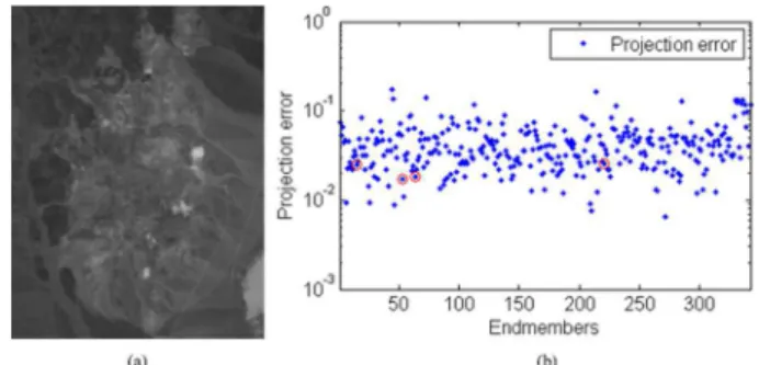
Fig. 7 Subimage and projection errors of real data: (a) band 30 (λ = 667.3 nm) of a subimage from the AVIRIS Cuprite Nevada dataset; (b) projection errors for all members onto this real dataset. The projection errors corresponding to these four materials are indicated by red circles.

validate the performance of hyperspectral unmixing algorithms. The scene comprises 224 spectral bands ranging from 0.4 to 2.5 μm, with a nominal spectral resolution of 10 nm. After removing low SNR and water absorption bands, 188 bands remain. The portion used in the experiments consists of 250×191 pixels. Figure 7 (a) shows this subimage at spectral band 30.

The spectral library used in this experiment is the same library A1 used in the previous simulated experiments, which contains 342 spectral signatures with 224 spectral bands.

From previous studies[10], [37], we know that this dataset contains four prominent materials, namely, alunite, buddingtonite, chalcedony, and montmorillonite. Fig- ure 7 (b) shows the projection errors obtained for all members onto this real dataset. The errors corresponding to these four materials are indicated by red circles. Here, the subspace projection method performs worse than in the simulated datasets because of various types of modeling error.

However, the projection errors corresponding to the four materials are still small. In experiments, the subspace di- mension inferred by HySime was 18. We set parameterTto be 82 to ensure all the endmember signatures are present in the reduced dictionary.

Figure 8 qualitatively compares the fractional abundances inferred by SUnSAL, CLSUnSAL, MUSIC-CSR, and the proposed algorithm for the four diﬀerent minerals.

The regularization parameter in this experiment was set as follows: 0.001 for SUnSAL, 0.05 for CLSUnSAL, 0.01 for MUSIC-CSR, and 0.5 for the proposed algorithm.

From Fig. 8, we can see that the fractional abundances estimated by the proposed algorithm are generally higher in the regions assigned to the respective materials in comparison to SUnSAL, CLSUnSAL and MUSIC-CSR. This is because the proposed algorithm considers the pruning strategy and sparsity enhancement strategy simultaneously. As a result of the pruning strategy, our pruned dictionary only contains 82 spectra signatures, successfully reducing the dictionary size by 76%. Thus, our proposed algorithm improves the accuracy of unmixing solutions.

Table 6 reports the average runtimes on the real hyperspectral dataset using the same computing environment as

(11)

Fig. 8 Fractional abundance maps estimated by SUnSAL, CLSUnSAL, and the proposed algorithm.

(Top to bottom) abundance maps for alunite, buddingtonite, chalcedony, and montmorillonite for (a) SUnSAL, (b) CLSUnSAL, (c) MUSIC-CSR, and (d) the proposed algorithm.

used for the simulated data. The runtime of the proposed algorithm is 39.02% of that of SUnSAL and is 11.21% of that of CLSUnSAL. Overall, our proposed algorithm is much

faster than the SUnSAL and CLSUnSAL algorithms, and is a little longer than MUSIC-CSR.

(12)

Table 6 Computation times for real data.

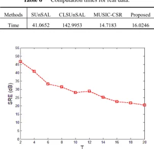
Fig. 9 Relationship between SRE andTin DC1 with SNR=30 dB for the proposed method.

5. Discussion

The greatest advantage of the proposed algorithm is the adoption of a dictionary pruning strategy, which can identify a subset of the library for unmixing. ThresholdT controls the size of the subset of the original spectral library. Fig- ure 9 shows the relationship between SRE andT in DC1 at SNR=30dB. Higher values ofT lead to lower SRE values.

However, when the dataset contains high levels of noise and the number of true signatures is large, thresholdTshould be set higher to avoid missing active signatures.

In the proposed algorithm, parameter λmust still be determined manually, which is a disadvantage. Hence, our future work will focus on how to automatically determine this parameter.

Although the results obtained using the proposed algorithm are very encouraging, the algorithm proposed in this paper is based on the LMM. In real hyperspectral images, nonlinearities do exist. Therefore, the nonlinear problem of mixed pixels should also be considered appropriately in the future design of the unmixing algorithm.

6. Conclusions

In this paper, we developed a hyperspectral unmixing method based on dictionary pruning and reweighted sparse regression. To mitigate the problems of high mutual coherence in spectral libraries, the algorithm identifies a subset of the original library elements using dictionary pruning strategy. The size of this subset is much smaller than that of the original library. To further improve the performance of unmixing method, we propose a weighted sparse regression algorithm called the W-CLSUnSAL algorithm. Thus, our proposed algorithm improves the accuracy of unmixing solutions while substantially reducing the average runtime.

Simulated and real hyperspectral data experiments showed that the proposed algorithm is more accurate and much faster than the SUnSAL and CLSUnSAL algorithms.

Acknowledgments

This study is financially supported by the National Key R&D Program of China (2017YFC0601505), Chinese Na- tional Natural Science Foundation (41672325, 41602334), the Leading talent training project of Neijiang Normal Uni- versity under 2017[Liu Yi-He]; the Innovative Team Pro- gram of the Neijiang Normal University under 17TD03;

the Sichuan province academic and technical leader training funded projects under 13XSJS002; the Foundation of Ph. D. Scientific Research of Neijiang Normal University under 2019[zhang shuang] and 2019[wang jiujiang].

References

[1] F. Li, M.K. Ng, and R.J. Plemmons, “Coupled segmentation and denoising/deblurring models for hyperspectral material identification,”

Numer. Linear Algebra Appl., vol.19, no.1, pp.153–173, 2012.

[2] X.-L. Zhao, F. Wang, T.-Z. Huang, M.K. Ng, and R.J. Plemmons,

“Deblurring and Sparse Unmixing for Hyperspectral Images,” IEEE Trans. Geosci. Remote Sens., vol.51, no.7, pp.4045–4058, 2013.

[3] G. Martin and J.M. Bioucas-Dias, “Hyperspectral Blind Reconstruc- tion from Random Spectral Projections,” IEEE J. Sel. Topics Appl.

Earth Observ., vol.9, no.6, pp.2390–2399, 2016.

[4] W. Tang, Z.W. Shi, Y. Wu, and C.S. Zhang, “Sparse unmixing of hyperspectral data using spectral a priori information,” IEEE Trans.

Geosci. Remote Sens., vol.53, no.2, pp.770–783, 2016.

[5] X.S. Liu, W. Xia, B. Wang, and L.M. Zhang, “An approach based on constrained nonnegative matrix factorization to unmix hyperspectral data,” IEEE Trans. Geosci. Remote Sens., vol.49, no.2, pp.757–772, 2011.

[6] L.N. Zhuang and J.M. Bioucas-Dias, “Fast hyperspectral image denoising and inpainting based on low-rank and sparse represen- tations,” IEEE J. Sel. Topics Appl. Earth Observ., vol.11, no.3, pp.730–742, 2018.

[7] J. Sigurdsson, M.O. Ulfarsson, J.R. Sveinsson, and J.M. Bioucas- Dias, “Sparse Distributed Multitemporal Hyperspectral Unmixing,”

IEEE Trans. Geosci. Remote Sens., vol.55, no.11, pp.6069–6084, 2017.

[8] Y.-Q. Zhao and J.X. Yang, “Hyperspectral image denoising via sparse representation and low-rank constraint,” IEEE Trans. Geosci.

Remote Sens., vol.53, no.1, pp.296–308, 2015.

[9] C.B. Li, T. Sun, K.F. Kelly, and Y. Zhang, “A compressive sensing and unmixing scheme for hyperspectral data processing,” IEEE Trans. Image Process., vol.21, no.3, pp.1200–1210, 2012.

[10] J.M. Bioucas-Dias, A. Plaza, N. Dobigeon, M. Parente, Q. Du, P.

Gader, and J. Chanussot, “Hyperspectral unmixing overview Geo- metrical, statistical and sparse regression-based approaches,” IEEE J. Sel. Topics Appl. Earth Observ., vol.5, no.2, pp.354–379, 2012.

[11] S.Z. Zhang, J. Li, H.C. Li, C.Z. Deng, and A. Plaza, “Spectral–

spatial weighted sparse regression for hyperspectral image unmixing,” IEEE Trans. Geosci. Remote Sens., vol.56, no.6, pp.3265–

3276, 2018.

[12] X.Q. Lu, H. Wu, Y. Yuan, P.K. Yan, and X.L. Li, “Mainfold regularized sparse NMF for hyperspectral unmixing,” IEEE Trans. Geosci.

[13] M.-D. Iordache, J.M. Bioucas-Dias, A. Plaza, and B. Somers, “Mu- sic-CSR Hyperspectral unmixing via multiple signal classification and collaborative sparse regression,” IEEE Trans. Geosci. Remote Sens., vol.52, no.7, pp.4364–4382, 2014.

(13)

[14] Y.T. Qian, S. Jia, J. Zhou, and A. Robles-Kelly, “Hyperspec- tral unmixing via L1/2 sparsity-constrained nonnegative matrix factorization,” IEEE Trans. Geosci. Remote Sens., vol.49, no.11, pp.4282–4297, 2011.

[15] J.M. Liu, C.X. Zhang, J.S. Zhang, H.R. Li, and Y.L. Gao, “Man- ifold regularization for sparse unmixing of hyperspectral images,”

Springerplus, vol.5, no.1, p.2007, 2016.

[16] C.Y. Zheng, H. Li, Q. Wang, and C.L.P. Chen, “Reweighted Sparse Regression for Hyperspectral Unmixing,” IEEE Trans. Geosci. Re- mote Sens., vol.54, no.1, pp.479–488, 2015.

[17] R. Heylen, J. Chen, M. Parente, and P. Gader, “A review of nonlinear hyperspectral unmixing methods,” IEEE J. Sel. Topics Appl. Earth Observ., vol.7, no.6, pp.1844–1868, 2014.

[18] J.M. Bioucas-Dias, “A variable splitting augmented Lagrangian approach to linear spectral unmixing,” Proc. 1st WHISPERS., pp.1–4, 2009.

[19] F.D.V.D. Meer and X.P. Jia, “Collinearity and orthogonality of endmembers in linear spectral unmixing,” Int. J. Appl. Earth Observ.

Geoinf., vol.18, no.1, pp.491–503, 2012.

[20] B. Somers, K. Cools, S. Delalieux, J. Stuckens, D.V.D. Zande, W.W.

Verstraeten, and P. Coppin, “Nonlinear hyperspectral mixture analysis for tree cover estimates in orchards,” Remote Sens. Environ., vol.113, no.6, pp.1183–1193, 2009.

[21] A. Halimi, Y. Altmann, N. Dobigeon, J.Y. Tourneret, P. Gader, A.J.

Plaza, and C.Y. Chi, “Nonlinear unmixing of hyperspectral images using a generalized bilinear model,” IEEE Trans. Geosci. Remote Sens., vol.49, no.11, pp.4153–4162, 2011.

[22] X.R. Zhang, C. Li, J.Y. Zhang, Q.M. Chen, J. Feng, L.C. Jiao, and H.Y. Zhou, “Hyperspectral Unmixing via Low-Rank Representation with Space Consistency Constraint and Spectral Library Pruning,”

Remote Sens., vol.10, no.2, p.339, 2018.

[23] Y.F. Zhong, R.Y. Feng, and L.P. Zhang, “Non-Local Sparse Unmix- ing for Hyperspectral remote sensing imagery,” IEEE J. Sel. Topics Appl. Earth Observ., vol.7, no.6, pp.1889–1909, 2014.

[24] W.-K. Ma, J.M. Bioucas-Dias, T.-H. Chan, N. Gillis, P. Gader, A.J.

Plaza, A. Ambikapathi, and C.-Y. Chi, “A signal processing per- spective on hyperspectral unmixing: insights from remote sensing,”

IEEE Signal Process. Mag., vol.31, no.1, pp.67–81, 2014.

[25] R. Wang, H.-C. Li, A. Pizurica, J. Li, A. Plaza, and W.J. Emery,

“Hyperspectral unmixing using double reweighted sparse regression and total variation,” IEEE Geosci. Remote Sens. Lett., vol.14, no.7, pp.1146–1150, 2017.

[26] D. Manolakis, C. Siracusa, and G. Shaw, “Hyperspectral subpixel target detection using the linear mixing model,” IEEE Trans. Geosci.

[27] J.M. Bioucas-Dias and M.A.T. Figueiredo, “Alternating direction algorithms for constrained sparse regression application to hyperspectral unmixing,” Proc. 2nd WHISPERS., pp.1–4, 2010.

[28] M.-D. Iordache, J.M. Bioucas-Dias, and A. Plaza, “Collaborative sparse regression for hyperspectral unmixing,” IEEE Trans. Geosci.

[29] M.-D. Iordache, J.M. Bioucas-Dias, and A. Plaza, “Hyperspectral unmixing with sparse group lasso,” IEEE Geosci. Remote Sens.

Symp., vol.24, no.8, pp.3586–3589, 2011.

[30] M.-D. Iordache, A. Plaza, and J.M. Bioucas-Dias, “On the Use of Spectral Libraries to perform Sparse Unmixing of Hyperspectral Data,” Proc. 2nd WHISPERS., pp.1–4, 2010.

[31] X. Fu, W.-K. Ma, T.-H. Chan, and J.M. Bioucas-Dias, “Self-Dic- tionary Sparse Regression for Hyperspectral Unmixing: Greedy Pur- suit and Pure Pixel Search Are Related,” IEEE J. Sel. Topics Signal Process., vol.9, no.6, pp.1128–1141, 2015.

[32] X. Fu, W.-K. Ma, J.M. Bioucas-Dias, and T.-H. Chan, “Semib- lind Hyperspectral Unmixing in the Presence of Spectral Library Mismatches,” IEEE Trans. Geosci. Remote Sens., vol.54, no.9, pp.5171–5184, 2016.

[33] A. Zare and P. Gader, “Sparsity promoting iterated constrained endmember detection in hyperspectral imagery,” IEEE Geosci. Remote

Sens. Lett., vol.4, no.3, pp.446–450, 2007.

[34] A. Huck and M. Guillaume, “Robust hyperspectral data unmixing with spatial and spectral regularized NMF,” Proc. 2nd WHISPERS., pp.1–4, 2010.

[35] M.-D. Iordache, J.M. Bioucas-Dias, and A. Plaza, “Sparse unmixing of hyperspectral data,” IEEE Trans. Geosci. Remote Sens., vol.49, no.6, pp.2014–2039, 2011.

[36] J.M. Liu, J.S. Zhang, Y.L. Gao, C.X. Zhang, and Z.H. Li, “Enhanc- ing spectral unmixing by local neighborhood weights,” IEEE J. Sel.

Topics Appl. Earth Observ., vol.5, no.5, pp.1545–1552, 2012.

[37] M.-D. Iordache, J.M. Bioucas-Dias, and A. Plaza, “Total variation spatial regularization for sparse hyperspectral unmixing,” IEEE Trans. Geosci. Remote Sens., vol.50, no.11, pp.4484–4502, 2012.

[38] M.-D. Iordache, J.M. Bioucas-Dias, and A. Plaza, “Dictionary pruning in sparse unmixing of hyperspectral data,” Proc. 4th WHISPERS., vol.49, no.6, pp.1–4, 2012.

[39] A. Erturk, M.-D. Iordache, and A. Plaza, “Sparse Unmixing With Dictionary Pruning for Hyperspectral Change Detection,” IEEE J.

Sel. Topics Appl. Earth Observ., vol.10, no.1, pp.321–330, 2017.

[40] J.M. Bioucas-Dias and J.M.P. Nascimento, “Hyperspectral Subspace Identification,” IEEE Trans. Geosci. Remote Sens., vol.46, no.8, pp.2435–2445, 2008.

[41] F.Y. Zhu, Y. Wang, B. Fan, G.F. Meng, and C.H. Pan, “Eﬀective spectral unmixing via robust representation and learning-based sparsity,” IEEE J. Sel. Topics Signal Process., vol.19, pp.1–13, 2014.

[42] A. Halimi, J.M. Bioucas-Dias, N. Dobigeon, G.S. Buller, and S.

Mclaughlin, “Fast hyperspectral unmixing in presence of nonlinearity or mismodeling eﬀects,” IEEE Trans. Comput. Imaging, vol.3, no.2, pp.146–159, 2017.

[43] E.J. Cand`es, M.B. Wakin, and S.P. Boyd, “Enhancing sparsity by reweighted L1 minimization,” J. Fourier Anal. Appl., vol.14, no.5-6, pp.877–905, 2008.

[44] F. Yin, “Study on the theory and method of linear hyperspectral unmixing and its application,” Doctoral dissertation, CDUT, 2016.

[45] S. Wang, T.-Z. Huang, X.-L. Zhao, G. Liu, and Y.G. Cheng, “Double Reweighted Sparse Regression and Graph Regularization for Hyper- spectral Unmixing,” Remote Sens., vol.10, no.7, p.1046, 2018.

Hongwei Han received the B.S. degree in Mathematics education from Yan’an University, Yanan, in 2002, and M.S. degree in electronics and communication engineering from Chengdu University of Technology, Chengdu, in 2009.

He is Currently completing a Ph.D in Geomath- ematics in Chengdu University of Technology.

His research interests include hyperspectral remote sensing image processing, Partial diﬀeren- tial equation and its application.

Ke Guo is currently a professor and doctoral supervisor in the Chengdu University of Tech- nology. He is academic and technical leader of sichuan province, and enjoys special subsidies from the state council government. He is currently the head of the teaching team of mathematics geology in sichuan province, and the head of the scientific research and innovation team of high-level resources and environment in sichuan province. He has long been engaged in the teaching and scientific research of quantita- tive evaluation and prediction of resources and environment.

(14)

Maozhi Wang received the B.S. degree in mathematics from Southwest Normal Uni- versity, Chongqing, in 1996, and M.S. degree in computer software and theory from the Uni- versity of Electronics Science and Technology of China, Chengdu, in 2003 and the Ph.D. degree in geo-detection and information technology from Chengdu University of Technology, Chengdu, in 2014. He is currently a researcher in Geomathematics Key Laboratory of Sichuan Province in Chengdu University of Technology.

His research interests include hyperspectral remote sensing image processing and its application.

Tingbin Zhang received the B. S. in Sur- veying and Mapping from Chang’ An Univer- sity (Xian China), M. S. in Mineral Resources and Geological Engineering from Chengdu Uni- versity of Technology (Chengdu, China) and Ph. D. in Geodesy and Survey Engineering from Southwest Jiaotong University (Chengdu, China). He is currently a professor in the Chengdu University of Technology. His current research interests include remote sensing of environment, remote sensing of resources, survey- ing and mapping, etc.

Shuang Zhang received the B.S. degree in Mathematics and Applied Mathematics from the Neijiang Normal University, Neijiang, China, in 2007, and the M.S. degree in Control Engineer- ing from the Institute of Optics and Electron- ics, Chinese Academy of Sciences, Chengdu, in 2011. He is currently pursuing the Ph.D. degree in electrical and computer engineering with the University of Macau, Macau, China. He has been an Assistant Professor in College of Com- puter Science, Neijiang Normal University. His current research interests include human body communication, Digital signal processing, and body sensor network.