PAPER Special Section on Network Virtualization and Network Softwarization for Diverse 5G Services
Scalable State Space Search with Structural-Bottleneck Heuristics for Declarative IT System Update Automation
Takuya KUWAHARA†a), Takayuki KURODA†b), Manabu NAKANOYA†c), Yutaka YAKUWA†d),Nonmembers, andHideyuki SHIMONISHI†e),Member
SUMMARY As IT systems, including network systems using SDN/NFV technologies, become large-scaled and complicated, the cost of system management also increases rapidly. Network operators have to maintain their workflow in constructing and consistently updating such complex systems, and thus these management tasks in generating system update plan are desired to be automated. Declarative system update with state space search is a promising approach to enable this automation, how- ever, the current methods is not enough scalable to practical systems. In this paper, we propose a novel heuristic approach to greatly reduce computation time to solve system update procedure for practical systems. Our heuris- tics accounts for structural bottleneck of the system update and advance search to resolve bottlenecks of current system states. This paper includes the following contributions: (1) formal definition of a novel heuristic func- tion specialized to system update for A* search algorithm, (2) proofs that our heuristic function is consistent, i.e., A* algorithm with our heuristics returns a correct optimal solution and can omit repeatedly expansion of nodes in search spaces, and (3) results of performance evaluation of our heuristics. We evaluate the proposed algorithm in two cases; upgrading running hypervisor and rolling update of running VMs. The results show that computation time to solve system update plan for a system with 100 VMs does not exceed several minutes, whereas the conventional algorithm is only applicable for a very small system.
key words: orchestration, task planning, system update automation, auto- mated planning, change management, model-based engineering, declara- tive provisioning, network function virtualization
1. Introduction
Recent development and wide acceptance of SDN [1],[2]
and NFV[3],[4]technologies have made network infrastruc- ture greatly flexible, i.e. deployment, modification, scale-in and out, as well as destruction of (virtual) network systems can be done in a software-defined way. Network functions, such as router, firewall, load-balancer, IDS/IPS, and so on, are deployed as a virtual entity on any available physical servers, rather than manually installing physical boxes into the system. Scaling-up the number of such functions, for instance, can be done by instructing orchestrators or NFV platform software, rather than purchasing any new hardware boxes. Researches on automation of NFV resource opti-
Manuscript received April 12, 2018.
Manuscript revised July 26, 2018.
Manuscript publicized September 20, 2018.
†The authors are with System Platform Research Laboratories, NEC, Kawasaki-shi, 211-8666 Japan.
a) E-mail: [email protected] b) E-mail: [email protected] c) E-mail: [email protected] d) E-mail: [email protected] e) E-mail: [email protected]
DOI: 10.1587/transcom.2018NVP0009
mization can be found in many literatures, such as [5], for example. In addition, in plumbing among these functions, there’s no need to physically wire among them, or set up complex VLAN/routing configurations with a lot of con- straints, but SDN technology enables ideal plumbing among these functions with arbitrary logical topology, appropriate path selection, and logical separation from other services, regardless of physical network installations. Optimization of co-design of NFV function placement and SDN route op- timization can also be found in many literatures, such as[6], for example.
These technologies have made operator’s tasks for de- ployment and maintenance of the system significantly ease and agile, however, these tasks have to be well-prepared for every situations. Workflows for deployment and mainte- nance tasks have to be carefully designed so that the order of each step in the workflow ensures no system failure nor effects on running services. This is an another burden for operators to design such workflows in advance of the ser- vice operation, as network systems become more complex and demands for network services adapted to allow diverse customization requirement. In addition, such pre-defined workflow can only be applied for well-prepared regular tasks, such as increasing the number of functions within a prepared resource pool, or preparing a new virtual network based with common templates. Let us suppose a case, when a resource pool in some small area has been exhausted and needs to al- locate extra resource in different area, there would be a man- ual configurations to fetch resource in remote area, set up a network path, or extend virtual network span to that area, re- configure service chain topology or job dispatch policy, etc.
Someone can imagine another case where any network hard- ware or service halted unexpectedly and simple switching to stand-by system is not applicable, or there’s any trouble at a single point of failure, the operator is urged to prepare recovery workflow on-demand as quickly as possible. We can also imagine a workflow to patch or upgrade hypervisor, which requires delicate treatment of services running on top of that hypervisor because such services have mutual effects with other services running at other part of the system.
Based on above discussions, we are facing to new fron- tier of SDN/NFV research towards automation of workflow generation. This will make manual and labor jobs of oper- ation expert fully automated and possibly autonomous self- management of a network infrastructure. In this paper, we discuss automated system update to eliminate human task Copyright © 2019 The Institute of Electronics, Information and Communication Engineers
of generation of system update plan. To this end, we are proposing to employDeclarative system update[7]–[12]for this issue. Taking this approach, system operators have only to inputthe desired system state, and planning engines au- tomatically generate system-update plans on behalf of the system operators.
Some declarative system update approaches [7], [8]
adopt a “state-space search” as an automated planning method. Although it has been suggested that a state space of a system grows exponentially with increasing number of sys- tem components[11], our previous work proposed a kind of a divide-and-conquer technique to solve planning problems concerning updating large-scale systems[8].
However, in some cases, exponential growth of the state space remains an issue concerning planning problems. Ac- cordingly, the notion ofglobal constraintswas introduced to planning system updates[12]. This notion makes it possi- ble to impose certain system requirements on the transient and desired states of a system update. For example, when system operators need to update a service that manages crit- ical infrastructure and cannot be stopped even during system update procedures, planning engines accounting for global constraints can generate a system-update plan while keeping the system operating normally.
Unfortunately, if we introduce global constraints to our previous approach, our divide-and-conquer strategy may not sufficiently break an original planning problem down to fine grained sub-problems. In such cases, system update would not be finished in realistic time, even if the size of the system is realistic, for example, consisting of 50∼100 components.
In our preliminary report, we have proposed a ba- sic method for efficient planning of declarative system up- date[13]. In this paper, we further propose complete method which can omit recomputation of values of heuristic func- tion to be more efficient and present mathematical proof of justification for this optimization. We also present various experimental results to verify the effectiveness of the method.
The proposed method suppresses the increase in time for planning and makes declarative system update a more powerful tool for system management. The proposed plan- ning method is based on the observation that most system up- dates containa “bottleneck” component, which takes many steps to update due to dependencies with other components.
We found that a system-update plan can be quickly formu- lated by setting the update of the bottleneck components as a priority. We formalized this finding asa heuristic function for the A* search algorithm, and we designed an efficient planning method tailored for declarative system update.
In the rest of this paper, related work is introduced in Sect. 2. In Sect. 3, declarative system update with state-space search is overviewed. In Sect. 4, state models and planning problems are formalized in the similar way to a reported method[8]. In Sect. 5, a heuristic function is formulated and validated, and an efficient algorithm for calculating that heuristic function is devised and validated. In Sect. 6, the results of an experimental evaluation of the performance of the algorithm are presented and discussed, and in Sect. 7, the
conclusions of this study are presented.
2. Related Work
A fundamental framework for declarative system update, which accepts a desired state as input and generates work- flows that execute system update by automatic planning, has been proposed by El Maghraoui et al.[11].
The planning technique used in[11]is calledpartial- order planning (POP). In short, a POP engine receives a set ofactions, which are elemental operations for system update (and similar tothe transitionsin our models), and constructs a partial plan.
In contrast to a totally ordered plan specifying a com- plete order of actions, a partial plan is a partially ordered set of actions and specifies only necessary and sufficient or- dering of actions. A partial plan can be more efficiently executed than a totally ordered plan because two or more actions can be executedin parallelwhen they are not related by their relative orders.
In a comparative study on several planning techniques, the most-suitable technique for planning an IT-system up- date was discussed[14]. It was concluded thathierarchical task network (HTN)algorithms, which decompose a high- level action into several finer-grained actions and finally el- ementary actions by applying decomposition to the actions hierarchically, are the most suitable.
It was also pointed that a general HTN algorithm is insufficient to solve a planning problem concerning a large- scale IT system. In another work, to tailor an HTN algorithm to IT system planning[15], a hybrid approach to a HTN and state-space search and several optimization were proposed [16].
In contrast to those works, in our previous work[8]–
[10], we chose state-space search for making it possible to explicitly deal with system states and easily taking global constraints (cf.[12]) into account. State-space search can be adapted to account for global constraints by restricting a state space to states satisfying given global constraints. This feature is difficult to integrate into methods such as those that handle states of IT systems implicitly (like POP and HTN).
As mentioned in Sect. 1, the size of state spaces grows exponentially with increasing number of components in a system. To address this issue, our previous work[8]adopted a divide-and-conquer strategy, namely, dividing systems into strongly connected components by dependencies. By our divide-and-conquer strategy, the main factor of scalability of a state-space search reduces from the size ofa whole sys- temto the maximum size ofstrongly connected components of a system. However, global constraints make related sys- tem components depend on each other, and our divide-and- conquer strategy does not work due to these dependencies.
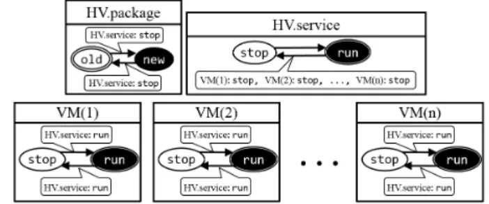
3. Illustration of Fully Declarative System Update This section illustrates declarative system update. Figure 1 shows our motivating example, that is a situation in whichn
Fig. 1 Motivating example: updating a running hypervisor.
Fig. 2 An example of state model planning.
virtual machines are hosted on a hypervisor and the hyper- visor needs to be stopped and restarted for version update.
In the rest of this section, for brevity, we assume thatn=1, that is, only one VM is hosted on the hypervisor.
In this example, it is supposed that the hypervisor can- not be upgraded while in operation and that the hypervisor cannot be stopped while it is hosting the VM. In this case, system update must be executed in correct order, namely, (1) stop the VM, (2) stop the hypervisor, (3) upgrade the hyper- visor, (4) restart the hypervisor, and (5) reboot the VM.
3.1 Modeling Systems
In this study, each system component is modeled by state models. State models consist of several transition systems with dependencies on their transitions. Here, a transition system consists ofstatesof a system andtransitionsbetween them, and represents behaviors of a system with discrete internal status.
System updates are modeled by the planning problems on state models, which is calledstate model planning. A state model planning is defined by a state model as well as initial and desired states of each transition system of the state model. Figure 2 shows an example modeled by state-model planning.
Each rectangle in the figure represents a transition sys- tem, henceforth calleda state element to emphasize that it isan elementof a whole state model. Each circle in a state element is a state of it, and each arrow between two states is a transition between them. Each double-lined state isan initial stateof each state element, and each filled-with-black
state is a desired stateof each state element. The goal of system update is for all components to transit from an initial state to a desired state.
In Fig. 2, three state elements are shown. “HV.package”
has two states,oldandnew, which represent an old version and a new version of the package of the hypervisor, respec- tively. “HV.service” has two states, runandstop, which represent running and stopped states of the hypervisor, re- spectively. “VM” also has two states,runandstop, which represent running and stopped states of the VM, respec- tively†.
In Fig. 2, some transitions have a label with a name of an element and its state. For example, the label “VM:stop”
is attached to the transition fromruntostopin HV.service.
These labels represent dependencieson transitions. A de- pendency on a transition representsa requirement to use the transition. That is, dependency “d:s” on a transition from srctodstof state elementemeans that “e’s state can move fromsrctodstonly if componentdis at states.”
We note that system operators do not have to directly represent a state model of their systems. Representing state model is equally or more time-consuming tasks for system operators. We assume that our declarative system update tool uses high-level models to hide details of states, tran- sitions and dependencies. For example, the component model[9],[10]is proposed, which consists of system com- ponents, connections between them, and property of them.
In this model, the model encapsulates the details of com- ponents and connections, and are converted into a detailed model that corresponds to the state model.
3.2 State Model Planning
The goal of state model planning is to discover the shortest sequence of transitions that transfers states of all compo- nents to desired states while keeping all requirements on labels fulfilled. A system-update plan is obtained as a so- lution of state model planning, and system update can be correctly performed by following the system-update plan.
For example, one solution of the problem shown in Fig. 2 is given as the following plan:
1. VM:run→stop 2. HV.service:run→stop 3. HV.package:old→new 4. HV.service:stop→run 5. VM:stop→run
(Here, notatione:a→bdenotes a transition fromatobin e.) This solution gives a correct system-update plan directly.
A way to formulate state-model planning as a shortest- path problem ona state graph, which is a transition system integrating all system components, was shown by Kuroda and Gokhale[8]. For example, Fig. 3 shows a state graph of our running example. A system-update plan can be found as
†Precisely, the “VM” component should be named
“VM.service”, but it is omitted for brevity.
Fig. 3 State graph of the system shown in Fig. 2.
paths from the initial state (1) to the desired state (5) over this state graph as the following path: (1)→(2)→(3)→(7)
→(6)→(5).
4. Formal Definitions
In this section, state models and state model planning are formalized.
4.1 Notations
The following useful notations are introduced first.
• LetIbe a set. When tupleX =(Xi)i∈I is an element of Q
i∈IXi, X[i] denotes Xi. That is, _[i] is an i-th projection map.
• Suppose thatI ={i1, . . . ,in}. TupleXsuch asX[i]= Xican also be denoted as{i1:Xi1, . . . ,in :Xin}.
• Sequence ofx1, . . . ,xnarranged in this order is denoted ashx1, . . . ,xni.
• Whens=hx1, . . . ,xni, length ofsis defined asnand denoted asksk.
4.2 State Model
System components are modeled as unlabeled transition sys- tems, which calledstate elements.
Definition 4.1(State element). A state elementeis defined as a pair(S,T)whereSis called states, and T ⊆S×Sis called transitions. Scan be denoted as S(e)andT can be denoted asT(e).
State elements of a state model represent behavior of components (i.e., finer-grained parts of systems), and the state model represents the behavior of the whole system that consists of these components. Thus, to formally define a state model, interactions between state elements, called
“dependencies”, need to be defined. For this purpose,global states and global transitionsof a set of state elements are first introduced.
Definition 4.2 (Global state and global transition).
LetEbe a set of state elements.
Global states overE are defined as a set of all tuples of states overE. Formally, global states SE are defined asQ
e∈ES(e).
Global transitions over E are all transitions S
e∈ET(e)extended to global states. Formally, let e ∈ E,t ∈ T(e)and σ1, σ2 ∈ SE. (σ1,t, σ2) is a global transition whent =(σ1[e], σ2[e])holds and σ1[e0]=σ2[e0]holds for eache0∈E\ {e}.
A set of all global transitions overEis denoted asTE, and(σ1,t, σ2)∈ TEis denoted astσ
1.
Intuitively, global states representstates of a whole system, and global transitions representcomponent-wise transitions of a whole system.
The notion ofdependencyamong state elements can be introduced as follows. As mentioned in Sect. 3.2, dependen- cies represent restrictions on transitions of state elements, such as “The VM instance can be launched only when the hypervisor is running.”
Definition 4.3(Dependency). LetEbe a set of state elements.
A dependency overEis a mappingDfrom each transition inE to a tuple of (non-empty) subsets of states inE:
D:t7→(Be)e∈E (whereBe⊆S(e)∧Be,∅) State element e is said to be depending to e0 when D(t)[e0] , S(e0) holds for some t ∈ T(e). Dependency frometoe0can be denoted ase
D e0. When it is clear from the context,Dcan be omitted, ande e0can be simply written.
A dependency maps from each transition to a set of global states that the transition is executable. Formally, A transition tis said to beexecutable at a global stateσwhenσ[e] is in D(t)[e] for alle∈ E.
The following notation is also introduced:
• A set of all dependencies overEis denoted asDE.
• When B[e] = S(e)holds, “e : S(e)” can be omitted from {e1 : B[e1],e2 : B[e2], . . . ,en : B[en]}for sim- plicity of expression.
• The symbol>denotes{e1 :S(e1), . . . ,en :S(en)}.
• When D is a dependency and (s,d) is a transition, D((s,d))can be denoted asD(s,d).
Then, state models are formally defined as follows. Let Ebe a set of state elements andDbe a dependency overE.
A state model is defined as pairM=(E,D).
Example 4.1. State elements of the system shown in Fig. 4 are formalized as follows:
• HV.package=({old,new},{(old,new)})
• HV.service=({runhv,stophv},
Fig. 4 State model of the system used in Sect. 3.
{(runhv,stophv),(stophv,runhv)})
• VM=({runVM,stopVM},
{(runVM,stopVM),(stopVM,runVM)})
DependencyDbetween these state elements is defined as
D(old,new)={HV.service:{stophv}}
D(runhv,stophv)={VM:{stopVM}}
D(runVM,stopVM)=D(stopVM,runVM)= {HV.service:{runhv}}
; otherwise,D(t)=>.
Finally, the state model of the system in Fig. 4 is given asM=({HV.package,HV.service,VM},D).
4.3 State Graph
As mentioned in Sect. 3.2, a state model is translated into one transition system called astate graph[8].
Definition 4.4(State graph). LetM =(E,D)be a state model. A state graph G(M) = (S,T) is a labeled state transition system defined as
• S=SE
• T =(
tσ ∈ TE
tis executable atσ.)
State graph is a graph whose nodes are states of a sys- tem, and edges are (executable) transitions between them.
A global transition(σ1,t, σ2) inT can be denoted as σ1→−t T σ2, or simplyσ1→−t σ2 whenT is clear from the context.
Example 4.2. LetM be a state model defined in the ex- ample 4.1. Figure 5 shows the state graph G(M), which consists of six global statesσ0, . . . , σ5. Here, “hv.p” (resp.
“hv.s”) abbreviates “HV.package” (resp. “HV.service”). In Fig. 5, two “unreachable” global states: (hv.p:new,hv.s: stophv,VM: runVM)and (hv.p: old,hv.s: stophv,VM: runVM)are omitted.
4.4 State Model Planning
State model planningand itssolutioncan now be defined.
Formally,state model planningis defined as a planning prob- lem defined for a state graph of a state model froma global initial statetoa global desired state.
Fig. 5 State graph of the state model shown in Fig. 4.
Definition 4.5(State model planning). State model planning is a tripleP=(M, σ0, σf).
• M: state model
• σ0 ∈ G(M): global initial state
• σf ∈ G(M): global desired state Pathson state models are defined as:
Definition 4.6 (Path on state models). Let M = (E,D) be a state model, and G(M) = (S,T) be the state graph of M. If σ0, σ1, . . . , σn ∈ S and t1,t2, . . . ,tn ∈ T satisfy the following relations:
σ0 −→t1 T σ1, σ1−→t2 T σ2, . . . , σn−1−−t→n T σn sequenceht1,t2, . . . ,tniis called a path onM from σ0toσn.
A solutionto state-model planning(M, σ0, σf)is de- fined as one of the shortest paths on M from σ0 to σf. Hence,L(P)denotes:
• the length of a solution to state model planningPwhen Phas a solution, or
• ∞whenPhas no solution.
By definition of a solution to state-model planning, a solution to state model planning(M, σ0, σf)can be obtained by solvingshortest path searchproblem defined for a graph G(M)fromσ0 toσf. A heuristic search algorithm, a.k.a.
the A* algorithm [17], is adopted to solve a shortest-path search problem defined for a state graph with the proposed heuristic function.
5. Heuristic Function for State Model Planning
5.1 Challenging Case in Realistic Use
For brevity of examples, we only discussed about a simple and small problem consisting a VM and a hypervisor so far.
However, in many cases, hypervisors manage two or more VMs. It is supported that n is taken as a natural number more than two, and n VMs are hosted on the hypervisor.
A state model of a system containingn VMs has 2n+1+2 global states. Unfortunately, in “hop count” measurement, the desired state of the running example is situated at the farthest point from the initial state of the running example.
Therefore, if Dijkstra’s algorithm[18]is used to find a path from an initial state to a desired state, then all over the global states are traversed and the problem will never be solved in a practical time whenn is large (e.g., whenn > 100).
Accordingly, to deal with large systems, a heuristic function tailored for state model planning must be adopted.
5.2 Critical Element Heuristic Function
The proposed heuristic function is based on the following observation. In many cases of system update, a “bottleneck”
component occurs in the entire system update. That is, a component has many dependencies to other components di- rectly or indirectly, and resolving its dependencies takes most of the updating time. The element of that bottleneck compo- nent is calledthe critical element. For example, in the system shown in Fig. 2, HV.package is said to be the critical element of the planning problem, because transferring states of all other elements are caused by the update of the HV.package.
The proposed heuristic function can be regarded as one of variants of relaxed planning heuristics[19]. That is, de- pendencies of a given state model planning are relaxed by extracting dependencies that only relate to the critical ele- ment and removing all other dependencies. The length of a solution of therelaxedstate model planning under approxi- mates that of the original problem. Thus, thisapproximate length of a solutioncan be used as an admissible heuristics of the A* search algorithm.
The critical element of given state model planning must be identified. The proposed algorithm searches for the crit- ical element by using abrute-forcealgorithm. Namely, for all elementse, given state model planning is relaxed bye, an approximate length of a solution is computed by solving each relaxed state model planning, and the element that pro- duces maximum approximate length is taken as the critical element.
5.3 Definition of Relaxation of State Model Planning and Critical Element Heuristic Function
First, e-derived dependency is introduced. Intuitively, e- derived dependency based on dependencyDis dependency Drestricted on a rooted tree whose root ise, nodes are E, and edges are a part of “ ” relations.
Definition 5.1 (e-derived dependency). Let M = (E,D)be a state model. A dependencyDe↓is called an e-derived dependency based onDwhen the fol- lowing conditions hold (1) - (4) for alle∈E:
(1) For each transition t and each state e0, D(t)[e0]⊆De↓(t)[e0]holds.
(2) eis not depended from any othere∈E. (3) DependencyDe↓does not form a cycle.
(4) ∀e1,e2,e3∈E\ {e}.
e2
De↓
e1∧e3 De↓
e1
⇒e2=e3
Fig. 6 State model planningPε.
Fig. 7 e1-rooted tree of dependencies overPε.
Example 5.1. ProblemPεshown in Fig. 6 is used in Sect. 5.
DependencyDεofPεis given as:
Dε(a1,b1) ={e2:{b2,c2},e4 :{b4}}
Dε(b2,a2) ={e3:{b3}}
Dε(a4,b4) ={e2:{a2},e3 :{b3}}
Dε(·,·) => (otherwise)
The following two e1-derived dependencies are introduced as 1) If all dependencies except for direct dependencies are removed frome1, the followinge1-derived dependencies Dεe↓1directare obtained:
Dεe↓1direct(a1,b1) ={e2 :{b2,c2},e4:{b4}}
Dεe↓1direct(·,·) => (otherwise)
2) If all dependencies except for those along with ane1- rooted tree of dependencies shown in Fig. 7 are removed, the followinge1-derived dependenciesDεe↓1derivedare obtained:
Dεe↓1
derived(a1,b1) ={e2 :{b2,c2},e4:{b4}}
Dεe↓1derived(b2,a2) ={e3 :{b3}}
Dεe↓1derived(·,·) => (otherwise)
relaxed state model and relaxed state-model plan- ningcan thus be defined on the basis of an e-derived de- pendency.
Definition 5.2 (Relaxed state model M |De↓ and re- laxed state-model planningP |De↓). LetM = (E,D) be a state model,ebe inE,De↓be ane-derived depen- dency,P=(M, σ0, σf)be a state model planning.
M |De↓ = (E,De↓)is called an De↓-relaxed state model of M and P |De↓ = (M |D↓e, σ0, σf) an De↓- relaxed state model planning ofP.
ProblemP |De↓is said to be arelaxedproblem ofPin the sense that a graphG(M)is a subgraph ofG M |De↓
. The problem P |De↓ takes only dependencies derived from einto account. Accordingly, a critical element and
critical element heuristics can be formally defined as fol- lows.
The following notation is introduced for brevity. Let P = (M, σ0, σf) be state model planning and σ be a global state ofM. P@σ is written for state-model plan- ning(M, σ, σf).
Definition 5.3. Critical-element heuristic function ϑP(σ):S →Nis defined as
ϑP(σ)=max
e∈E L(P |De↓@σ) Elementarg max
e∈E
L(P |De↓)is called a critical element ofP. (SubscriptPis omitted fromϑPandϑis simply written when it is clear from context.)
The following theorem shows that the function ϑ is consistent. Consistency is important property for heuristic functions in the following two points; (1) a consistent func- tion is also an admissible function, which guarantees A*
algorithm calculates a collect shortest path, and (2) values of a consistent function are invariant through A* algorithm.
We can optimize A* algorithm using this property.
Theorem 5.1. LetPbe state-model planning. FunctionϑP
is consistent, namely, ϑP(σ)≤ϑP(σ0)+1
holds for all global statesσ, σ0such asσ→σ0.
Proof. Letec,ec0 be critical elements of P@σ,P@σ0 re- spectively. When no path from σ0 toσf exists onP |De↓c, ϑP(σ0) = ∞and Theorem 5.1 holds. Therefore, the case that a path fromσ0toσf exists onP |De↓cis considered.
The shortest pathπonP |De↓c fromσ0toσf is chosen.
Because transitiontsuch thattσ =(σ,t, σ0)exists, pathπ0 exists on P |De↓c such thatt,t0,t1, . . . ,tn
| {z }
π
. Because ϑ(σ) is the length of the shortest path fromσtoσf onP |De↓c, the following equation is obtained:
ϑ(σ)≤ |π0|=|π|+1 (1)
Becauseec0 is a critical element ofP |De↓@σ0, the fol- lowing holds:
L(P |De↓c@σ0)≤L(P |De↓0c@σ0) (2)
|π| ≤ϑ(σ0) (3)
By (1) and (3),ϑ(σ)≤ϑ(σ0)+1 holds.
Theconsistencyproperty makes the proposed algorithm more efficient by eliminating recalculation of the value of the proposed heuristic function. The detail of optimization of A* search algorithm is discussed below.
5.4 Algorithm for Computingϑ(σ)
An algorithm for computing L(P |De↓@σ) for calculating
ϑ(σ) is proposed in the following. We fixe-deriving de- pendencies for each e in the rest of this section, and for brevity, P |De↓is abbreviated asP |e.
We note that the number of states of each state element is assumed to be enough small (e.g., 2∼5) to finish the pre- process explained in the following subsection in negligibly short time to whole planning process.
5.4.1 Preprocess
First, the proposed algorithm requiressimplee-local paths of each element e. Here,ane-local pathis a sequence of transition: (s0,d0),(s1,d1), . . . ,(sk,tk) ∈ T(e) such that di−1 = si holds for all i, and a local path is said to be simplewhen it visits each state at most once. Second, the algorithm requires the length of the shortest e-local paths of each elemente. Note that since shortest local paths are simple, these values can easily be obtained after all simple e-local paths of each elementeare obtained.
Before A* search algorithm is executed, the following preprocesses are executed. Allsimplee-local paths of each state pair(s,s0)in each elementeare calculated, and stored in an arrayspe. Then the shortest path of each state pair(s,s0) is obtained by choosing the shortest path fromspe[s,s0], and its length in an arraydiste.
Example 5.2. LetPε|e1bePε|Dεe1
↓derived. After the preprocess is applied toP |e, the following prerequisite data is obtained.
(spe[s,s]={hi}anddiste[s,s]=0are omitted for alle.)
• ei (i=1,3,4):
spei[s,s0]={h(s,s0)i},distei[s,s0]=1 (for alls,s0s.t. s,s0)
• e2:
spe2[b2,a2]={h(b2,a2)i,h(b2,c2),(c2,a2)i}, spe2[a2,c2]={h(a2,b2),(b2,c2)i},
spe2[c2,b2]={h(c2,a2),(a2,b2)i},
spei[s,s0]={h(s,s0)i} (for all others,s0s.t. s,s0)
diste2[a2,c2]=diste2[c2,b2]=2
diste2[s,s0]=1 (for all others,s0s.t. s,s0) 5.4.2 Main Algorithm
The value ofϑP(σ)is the maximum value ofL(P |ep@σ) for all states inP. In the proposed algorithm for calculating the value of ϑP(σ), all of the values of L(P |ep@σ) are calculated by the following algorithmcalc(P,e,σ):
FunctioncostOn(P,e,R) calculates the minimum cost of transferring states ofeand its dependent elements from initial states to desired states under a requirementR one.
Here, a requirement on an elementeis a sequence of a set of states ofe. Under requirementhR1, . . . ,Rmi,eneeds to visit one required state in eachRiin the order ofR1, . . . ,Rm.
Algorithm 1“calc(P,ep,σ)”: CalculateL(P |ep@σ)
1: fore∈Edo 2: visit[e]←false 3: end for
4: L←costOn(P |ep,e,σ,hi) 5: fore∈Edo
6: if notvisit[e]then
7: L←L+diste(σ[e], σf[e]) 8: end if
9: end for 10: return L
Algorithm 2“costOn(P,e,σ,hR0,R1, . . . ,Rmi)”
1: visit[e]←true 2: spc← ∞
3: forhs0,s1, . . .,smi ∈trace(hR0, . . .,Rmi)do
4: forπ∈pathThrough(σ0[e],s0,s1, . . .,sm, σf[e])do 5: spc0← kπk
6: fordep∈ {e0|e e0}do 7: req←pathReqs(P,dep, π) 8: spc0←spc0+costOn(P,dep, σ,req) 9: end for
10: ifspc>spc0thenspc←spc0 11: end for
12: end for 13: return spc
AlgorithmcostOnis defined asAlgorithm 2.
Functiontrace(hR0, . . . ,Rmi)returns a set of sequences of states and be formally defined as:
trace(hi)={hi},trace(hR0, . . . ,Rmi)=R0× · · · ×Rm Function pathThrough(s0,s1, . . . ,sk) returns e-local paths from s0 to sk visiting s0,s1, . . . ,sk and be formally defined as:
pathThrough(s0,s1, . . . ,sk)
={concatenation ofπ1, . . . , πk
|π1 ∈spe[s0,s1], . . . , πk ∈spe[sk−1,sk]}
FunctionpathReqs(P,e,π) returns a requirement that is a sequence consisting of dependencies ofπand be formally defined as:
pathReqs(P,e, π)=hD(t10)[e], . . . ,D(t0l)[e]i
whereht10, . . . ,tl0i: a sequenceπwith all>removed Finally, the valueϑPε(σ)is obtained as the maximum value ofcalc(Pε,e, σ)for alle.
Example 5.3. LetPε|e1=(M, σ0, σf)bePε|Dεe↓1
derived. First, an execution process of costOn(Pε|e1,e1, σ0,hi) is shown below. In the following explanation, for simplicity, we omit common argumentsPε|e1andσ0incostOn(Pε|e1,e, σ0, π) and simply writecostOn(e, π).
First,costOncalls two recursive calls of itself:
costOn(e1,hi)
=costOn(e4,h{b4}i)+costOn(e2,h{b2,c2}i)+kh(a1,b1)ik
The value ofcostOn(e4,h{b4}i) is calculated immedi- ately: costOn(e4,h{b4}i)=kh(a4,b4),(b4,a4)ik=2.
In the calculation of the value ofcostOn(e2,h{b2,c2}i), The cost of paths h(a1,b1),(b1,c1),(c1,a1)i and h(a1,b1), (b1,a1)iare compared in line 10, and returns the smaller as the value ofcostOn(e2,h{b2,c2}i).
costOn(e2,h{b2,c2}i)
=min{kh(a1,b1),(b1,c1),(c1,a1)ik,
costOn(e3,h{b3}i)+kh(a1,b1),(b1,a1)ik}
=min{3,kh(a3,b3),(b3,a3)ik+2}=min{3,2+2}=3 Finally, the value ofcostOn(e1,hi)is calculated as:
costOn(e1,hi)
=costOn(e4,h{b4}i)+costOn(e2,h{b2,c2}i)+kh(a1,b1)ik
=2+3+1=6
In the above execution process, each visit[e]is set to truefor alle. Thus,calc(Pε,e1, σ0)returns6, which is the return value ofcostOn(Pε|e1,e1, σ0,hi).
5.5 Optimize A* Search with Critical Element Heuristics The A* search algorithm was proposed by Hart et al.[17]and is described asAlgorithm 3. Here, the detail of backtracking procedure for picking up the found path is omitted for brevity.
Algorithm 3“A*(G = (S,T),s0,sf,h)”: Search the shortest path on the graphG=(S,T)froms0tosfwith the heuristics h
1: cost[s0]←h(s0); Open.add(s0) 2: whileOpen,∅do
3: smin←arg min s∈Open
f(s)
4: ifsmin=sf thenreturn a shortest path obtained by backtracking.
5: Open.remove(smin); Closed.add(smin) 6: forn: all neighbor nodes ofsdo 7: f(n)←cost[smin]−h(smin)+h(n)+1 8:
if(n<Open∧n<Closed)
∨(n∈Open∧f(n)<cost[n])
∨(n∈Closed∧f(n)<cost[n])then 9: cost[n]←f(n); Open.add(n) 10: end if
11: end for 12: end while
Additionally, we can adopt the following optimization techniques of A* search algorithm andϑ:
1) According to Theorem 5.1, the value f(s)inAlgo- rithm 3is not updated. Therefore, the calculation in lines 7−9 ofAlgorithm 3can be omitted whenn∈Closed.
2) A tie breakingtechnique can be adopted. That is, smincan be freely chosen from nodes whose cost is minimum in all nodes in Open in line 3 ofAlgorithm 3. The proposed algorithm choose the farthest node tos0.
3) When∀t,e.De↓1(t)[e] ⊆De↓2(t)[e] holds, we can re- movee1from the candidates of critical elements. Addition- ally, when σ[e1] = σf[e1] and ∀t < T(e1).De↓1(t)[e] ⊆ De↓2(t)[e] hold for all e, we have L(P |De↓1@σ) ≤ L(P |De↓2@σ) and have only to calculate the value of L(P |De↓2@σ).
4) Amemoizationtechnique can be adopted. Because pathReqsis often called many times with the same argu- ments, the result of eachpathReqscall is stored and reused.
5) Let P = (M, σ0, σf) be a state model planning.
When we regard a state model M as a graph with nodes of state elements and edges of dependencies, the graph of M is sometimes divided into some connected components C1,C2, . . . ,Ck and we can construct an another state model planningPiby restrictingPover state elements of eachCi. Then, we can use more (or equal) accurate heuristics than ϑ. That is, we adopt sum of values ofϑPi(σ)for eachPi instead of the value ofϑP(σ).
Finally, the optimizedAlgorithm 3provides a system- update plan, P = (M, σ0, σf), as the return value of A*(M, σ0, σf, ϑP).
6. Performance Evaluation
We applied the proposed algorithm to solve system update plan of SDN/NFV systems. We start with very basic exam- ples to safely upgrade running hypervisor without risking VMs, or virtual network functions, running on top of the hypervisor. And we also tested the algorithm for a system that needs rolling update to avoid fatal incidents and zero downtime update for high availability.
We implemented our heuristic functionϑwithDe↓derived
in Scala and evaluated performance of our planning algo- rithm that uses critical element heuristics. Experiments were conducted on a machine with Intel(R) Xeon(R) E5-1620 0 (3.60GHz, 32GB memory) with timeout of 1 hour. We use scala runtime options “-J-Xms16G -J-Xmx16G” in perform- ing all experiments.
6.1 Upgrade of Running Hypervisor
As we mentioned in the prior sections, the problem shown in Fig. 1, which is to upgrade a hypervisor, is a difficult problem for declarative system update because this induces search in state space of exponential size. Our first experiment is performed on the problem shown in Fig. 1, which includes a hypervisor andnVMs.
Figure 8 depicts the state model planning HV-VM(n), which is a state model representing the system of Fig. 1. The state model planningHV-VM(n)is similar to our motivating example shown in Fig. 2 but hasn(>1)VMs. The current state ofHV-VM(n) is that the hypervisor of the old version package is hostingn VMs and the desired state is that the hypervisor is hostingnVMs similarly but the package of the hypervisor is updated.
Fig. 8 HV-VM(n): planning problem of updating a hypervisor.
Fig. 9 A load balanced cluster.
6.2 Rolling Update
As we mentioned in Sect. 1, in system updates, operators are often urged to design workflows so that the system update raise no fatal incidents of running services. If a system con- sists of two more VMs installed the same function, operators can adoptrolling update strategyto update these VMs with no downtime. Namely, in rolling update strategy, operators will not update all VMs simultaneously, but onlysubsetof VMs at a time.
Figure 9 shows a load balanced cluster, which is an example of system that we can update each VMs by rolling update. V M(1), V M(2), ..., andV M(n) are application servers where the same application is installed. The load balancer distributes attached VMs and, in most cases, all VMs are necessarily needed to keep a service in operation.
Therefore, if the enough number of VMs is in operation, the service on Fig. 9 keeps alive even in system update.
Figure 10 shows the state model planningRolling(n), which represents system update in Fig. 9 withnVMs. The load balancer is not appeared in Rolling(n) because the state of the load balancer doesn’t affect the update and ap- parently keeps in the “running” state. Here, we note that Fig. 10 doesn’t take the condition for keeping service run- ning into account. In order to obtain rolling update plans, we need to add a kind of global condition to the planning prob- lemRolling(n)and solve the problem with the additioncal condition. We add the condition that “at leastm(>0)VMs are running” to the problemRolling(n). Our planner can easily deal with such an additional conditions by excluding global states violating the condition.
Fig. 10 Rolling(n): planning problem of rolling update.
6.3 Zero Downtime Updates of ToR Switches in a Data Center
We consider an another example such that uses standby com- ponents for update. As we mentioned in Sect. 1, declarative system update tools uses extra resources and standby com- ponents when system update cannot be completed in main systems. Let us suppose a case of duplicated ToR switches in a data center. Important network appliances, including ToR switches, are often duplicated for high availability. Even when main switches fall down, standby switches activate as a substitute for the main switch and keep servers mounted on the rack accessible. Additionally, even in firmware update of ToR servers with requireing system reboot, the update can be completed with no downtime by detouring traffic to standby switches.
Figure 11 shows the latter case. There are n racks with eight servers and two ToR switches. In each rack, one ToR switches is an active switch, and other is a standby switch. Now, the administrator plans firmware update of active switches with no downtime.
Figure 12 shows a part of state model planning of Fig. 11, which represents just one pair of active- standby switch and contains state elements that show a firmware of active switch (SW[i].main.firmware), ser- vices of active and standby switch (SW[i].main and SW[i].sub), routing (SW[i].routeBy), connection to core switch (SW[i].connection), and connection to each server (SW[i,1].connection, · · ·, SW[i,8].connection). The state model planning UpdToR(n) is defined by n switch pairs SW[1],SW[2], . . . ,SW[n]. Similarly to Rolling(n), we need to add global condition that “all switches keep con- nection among connecting components”. That is, all state elements of “.connection” keep in the state “on”.
6.4 Results
The line graph Fig. 18 shows the results of experiments to solveHV-VM(n) by Dijkstra algorithm and our method.
Fig. 19 shows the results of experiments usingRolling(n)
Fig. 11 A network system on a data center.
Fig. 12 A state model planning of active/standby switches ofUpdToR(n).
Plan
1. VM(1):run →stop 2. VM(2):run →stop 3. VM(3):run →stop 4. HV.service:
run →stop
5. HV.package:old→new 6. HV.service:
stop →run 7. VM(1):stop →run 8. VM(2):stop →run 9. VM(3):stop →run
Workflow 1. Stop VM(1) 2. Stop VM(2) 3. Stop VM(3) 4. Stop hypervisor 5. Upgrade hypervisor 6. Restart hypervisor 7. Restart VM(1) 8. Restart VM(2) 9. Restart VM(3)
Fig. 13 A plan forHV-VM(3)and a workflow for Fig. 1 ofn=3.
with the condition that “at least 1 VMs are running”. The horizontal line showsn and the vertical one shows elapsed time in seconds to find a solution of each problem. The line of “no heuristic” shows results of Dijkstra algorithm and the line of “our method” shows results of A* algorithm with critical-element heuristic function.
The line graph Fig. 18 shows that the computing time of state space search using Dijkstra algorithm drastically increases and exceeds an hour withn=24 on one hand. On the other hand, our method can calculate a plan even with n=100 in 5 minutes.
Figure 13 shows a plan for HV-VM(3) and the corre- sponding workflow. The plan correctly avoid accidental system stop by stopping the underlying hypervisor.
The results of experiments using Rolling(n) shows us striking difference of efficiency between two algorithm.
The line graph Fig. 19 shows the computing time of state
Plan
1. VM(1).attachment:
detached →attached 2. VM(1).service:run→stop 3. VM(1).version:old →new 4. VM(1).service:stop →run 5. VM(1).attachment:
attached →detached 6. VM(2).attachment:
detached →attached 7. VM(2).service:run→stop 8. VM(2).version:old →new 9. VM(2).service:stop →run 10. VM(2).attachment:
attached →detached
Workflow
1. Detach VM(1) from load bal- ancer
2. Stop VM(1) 3. Update VM(1) 4. Restart VM(1)
5. Attach VM(1) to load balancer 6. Detach VM(2) from load bal-
ancer 7. Stop VM(2) 8. Update VM(2) 9. Restart VM(2)
10. Attach VM(2) to load balancer
Fig. 14 A plan forRolling(2)and a workflow for Fig. 9 ofn=2.
Plan
1. SW[1].sub:off →on 2. SW[1].routeBy:main →sub 3. SW[1].main:on→off 4. SW[1].main.firmware:old→
new
5. SW[1].main:off →on 6. SW[1].routeBy:sub →main 7. SW[1].sub:on →off
Workflow
1. Activate standby switch SW[1].sub 2. Switch route from SW[1].main
to SW[1].sub 3. Stop SW[1].main
4. Update firmware of SW[1].main 5. Activate SW[1].main 6. Switch route from SW[1].sub
to SW[1].main 7. Stop SW[1].sub
Fig. 15 A plan forUpdToR(1)and a workflow for Fig. 11 ofn=1.
space search using Dijkstra algorithm drastically increases and exceed an hour withn = 10 whereas our method can calculate a plan even withn=100 in 10 minutes.
Figure 14 shows a plan forRolling(2)and the corre- sponding workflow. From begining step 1 to finishing step 5, VM(2) keeps in operation and from begining step 6 to fin- ishing step 10, VM(1) keeps in operation. Therefore, while performing this workflow, the load balancer can distribute workload to at least one of VM(1) and VM(2) and the system of Fig. 9 keeps alive even during the update.
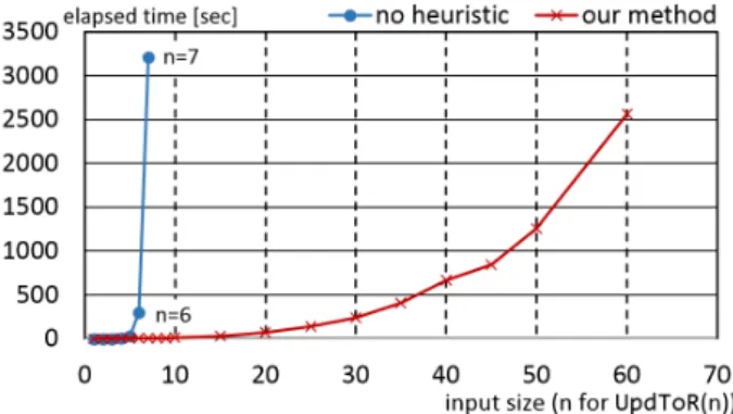
The line graph Fig. 20 also shows that notable differ- ence between Dijkstra algorithm and our heuristic search.
The computing time of state space search using Dijkstra algorithm exceeds an hour with n = 8 on one hand. On the other hand, our method can calculate a plan even with n=60.
Figure 15 shows a plan forUpdToR(1) and the corre- sponding workflow. From begining step 1 to finishing step 7, core switch and servers in the rack 1 keep connected. There- fore, while performing this workflow, the rack 1 in Fig. 11 keeps in operation.
6.5 Evaluation of Estimated Path Length byϑ
In the above experiments, our heuristic function can estimate precise value of shortest paths of these inputs by calcutating its value of global initial states. That is, our heuristics esti- mated length of solution ofHV-VM(n)as 2n+3,Rolling(n) as 5n, and UpdToR(n)as 7n at global initial states of each problem. We note that becauseRolling(n)(orUpdToR(n))
Fig. 16 The computation ofϑHV-VM(2).
Fig. 17 Example problemPcthatϑPc(σ0),L(Pc).
Fig. 18 The results of experiments usingHV-VM(n).
Fig. 19 The results of experiments usingRolling(n).
can be separated into sub-problemsPicorresponding to each VM(i) (or SW[i]), as me mentioned in Sect. 5.5, we use P
iϑPi(σ)instead ofϑRolling(n)(σ)(orϑUpdToR(n)(σ)).
Figure 16 illustrates computation ofϑHV-VM(2)by show- ing the value of L(HV-VM(2)|De↓derived) ande-rooted trees of De↓derived for each elementeinHV-VM(2). The critical el- ement of HV-VM(2) is HV.package because it follows the maximum value ofL(HV-VM(2)|De↓derived).
In contrast, we introduce an example problemPc that ϑPc(σ0) ,L(Pc)by Fig. 17. Any relaxedPchavestrictly shortersolution than the originalPc. Because any derived dependencies cannot depend on both e4.b4 ande4.c4, solu- tions of any relaxed problems don’t pass throughe4.b4and