RIMS Preprint No. 1470, Kyoto University
A Two-Sided Discrete-Concave Market with Possibly Bounded Side Payments: An Approach by Discrete
Convex Analysis
Satoru Fujishige and Akihisa Tamura August, 2004; Revised April, 2005
Abstract
The marriage model due to Gale and Shapley and the assignment model due to Shapley and Shubik are standard in the theory of two-sided matching markets. We give a common generalization of these models by utilizing discrete concave functions and considering possibly bounded side payments.
We show the existence of a pairwise stable outcome in our model. Our present model is a further natural extension of the model examined in our previous paper (Fujishige and Tamura [12]), and the proof of the existence of a pairwise stable outcome is even simpler than the previous one.
Satoru Fujishige
Research Institute for Mathematical Sciences, Kyoto University, Kyoto 606-8502, Japan.
phone: +81-75-753-7250, facsimile: +81-75-753-7272 e-mail: [email protected].
Akihisa Tamura
Department of Mathematics,
Keio University, Yokohama 223-8522, Japan.
phone: +81-45-566-1439, facsimile: +81-45-566-1642 e-mail: [email protected].
1. Introduction
The marriage model due to Gale and Shapley [14] and the assignment model due to Shapley and Shubik [28] are standard in the theory of two-sided matching markets. The largest difference between these two models is that the former does not allow side payments or transferable utilities whereas the latter does (see Roth and Sotomayor [26]).
Since Gale and Shapley’s paper a large number of variations and extensions have been proposed. Recently, the marriage model was extended to frameworks in combinatorial optimization. Fleiner [9] extended the marriage model to the frame- work of matroids, and Eguchi, Fujishige and Tamura [5] extended this formulation to a more general one in terms of discrete convex analysis which was developed by Murota [20, 21, 22]. Alkan and Gale [2] and Fleiner [10] also generalized the marriage model to another wide frameworks. The existence of stable matchings in these models are guaranteed.
For the other standard model, the assignment model, Kelso and Crawford [18]
proposed a seminal one-to-many variation in which a payoff function of each worker is strictly increasing (not necessarily linear) in a side payment, and a payoff func- tion of each firm satisfies gross substitutability and is linear in a side payment.
They showed the existence of a stable outcome.
On the other hand, progress has been made toward unifying the marriage model and the assignment model. Crawford and Knoer [3] extended Gale and Shapley’s deferred acceptance algorithm for the marriage model to the assignment model. Kaneko [17] formulated a general model that includes the two by means of characteristic functions, and proved the nonemptiness of the core. Roth and Sotomayor [27] proposed a general model that also encompasses both and inves- tigated the lattice property for payoffs. Eriksson and Karlander [6] proposed a hybrid model of the marriage model and the assignment model. In the Eriksson- Karlander model, the set of agents is partitioned into two categories, one for “rigid”
agents and the other for “flexible” agents. Rigid agents do not get side payments, that is, they behave like agents in the marriage model, while flexible agents be- have like ones in the assignment model. Sotomayor [31] also further investigated this hybrid model and gave a non-constructive proof of the existence of a pair- wise stable outcome. Fujishige and Tamura [12] proposed a generalization of the
hybrid model due to Eriksson and Karlander [6] and Sotomayor [31] by utilizing M\-concave functions which play a central role in discrete convex analysis.
The model in [12] motivates us to consider a more natural common gener- alization of the marriage model and the assignment model by utilizing discrete convex analysis. Our goal is to propose such a model which includes models due to Gale and Shapley [14], Shapley and Shubik [28], Eriksson and Karlander [6], Sotomayor [31], Fleiner [9], Eguchi et al. [5], and Fujishige and Tamura [12] as special cases, and to verify the existence of a pairwise stable outcome. The char- acteristic idea of our present model is to adopt a range of a side payment for each pair of agents instead of using the concept of rigid and flexible pairs. Our model can deal with rigidity and flexibility of pairs as ranges [0,0] and (−∞,+∞) of side payments respectively as well as any ranges of side payments. This approach is more natural and adaptable than that adopting rigidity and flexibility. Further- more, our proof for the existence of a pairwise stable outcome is simpler than that in our previous paper [12].
As we will discuss in Section 2, gross substitutability and M\-concavity are equivalent for set functions. It is our contribution in contrast to the results of Kelso and Crawford [18] that the existence of pairwise stable outcome is preserved in a many-to-many variation with quasi-linear workers’ payoff functions as well as its extensions with multi-units of labor time and possibly bounded side payments.
Moreover, we give not only a general mathematical model but also a new concrete common generalization of the marriage and assignment models. We call it the assignment model with possibly bounded side payments, which is the simplest common generalization. It seems that this model has not been studied in the literature. The existence of a pairwise stable outcome of this model is a direct consequence of our main result.
The present paper is organized as follows. Section 2 explains M\-concavity to- gether with some examples and gives its nice properties and several useful lemmas from the viewpoint of mathematical economics. Section 3 describes our general model and two concepts of stability, namely “pairwise stability” and “pairwise strict stability,” discusses relations between these two concepts, and gives our main theorem about the existence of pairwise stable outcomes. Proofs of prelimi- nary lemmas and theorems are put in Section 6, and a proof of our main theorem
is given in Section 5. Section 4 discusses relations between several existing models and our general model. In Section 5 we present an algorithm for finding a pairwise strictly stable outcome and prove its correctness, which shows our main theorem about the existence of a pairwise stable outcome. In Section 6 we give proofs of the lemma and theorems appearing in Section 3. Section 7 gives future work and open problems.
2. M
\-concavity
In this section we explain the concept of M\-concave function, which plays a central role in discrete convex analysis (see [22] for details). Let E be a nonempty finite set, and let 0 be a new element not inE. We denote by Z the set of integers, and by ZE the set of integral vectors x = (x(e) | e ∈ E) indexed by E, where x(e) denotes thee-component of vector x. Also, R and RE denote the set of reals and of real vectors indexed byE, respectively. Let 0 and 1 be vectors of all zeros and all ones of an appropriate dimension. We define the positive support supp+(x) and the negative support supp−(x) of x∈ZE by
supp+(x) ={e∈E |x(e)>0}, supp−(x) = {e∈E |x(e)<0}.
For each S ⊆ E, we denote by χS the characteristic vector of S defined by:
χS(e) = 1 if e ∈ S and χS(e) = 0 otherwise, and write simply χe instead of χ{e}
for alle∈E. We also define χ0 as the zero vector in ZE, where we assume 0∈/ E.
ForS ⊆E andx∈ZE, let x(S) = Pe∈Sx(e). For a vectorp∈RE and a function f :ZE →R∪ {−∞}, we define functions hp, xiand f[p](x) in x∈ZE by
hp, xi= X
e∈E
p(e)x(e), f[p](x) =f(x) +hp, xi (∀x∈ZE).
We also define arg max, the set of maximizers, of f on U ⊆ZE and the effective domain of f by
arg max{f(y)|y∈U}={x∈U | ∀y∈U : f(x)≥f(y)}, domf ={x∈ZE |f(x)>−∞}.
We abbreviate arg max{f(y)|y∈ZE} to arg maxf.
A function f : ZE → R ∪ {−∞} with domf 6= ∅ is called M\-concave (Murota [22] and Murota and Shioura [23]) if it satisfies
- 6
e e0
ZZ ZZ
ZZ ZZ
ZZ ZZ
ZZuhZ
x
u
y h
u u
e e
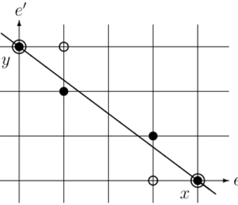
Figure 1: M\-concavity for two dimensional case: the sum of function values of black points or that of white points is greater than or equal to that of x and y.
(M\) ∀x, y ∈domf,∀e∈supp+(x−y), ∃e0 ∈supp−(x−y)∪ {0} : f(x) +f(y)≤f(x−χe+χe0) +f(y+χe−χe0).
((M\) is denoted by (−M\-EXC) in Murota [22].) Condition (M\) says that the sum of the function values at two points does not decrease as the points symmetrically move one or two step closer to each other on the set of integral lattice points of ZE (see Figure 1). This is a discrete analogue of the fact that for an ordinary concave function the sum of the function values at two points does not decrease as the points symmetrically move closer to each other on the straight line segment between the two points.
By the definition of M\-concavity, if f is M\-concave, then f[p] is also M\- concave for any p∈RE. Here are two simple examples of M\-concave functions.
Example 1: For the independence familyI ⊆2E of a matroid onE andw∈RE, the function f :ZE →R∪ {−∞} defined by
f(x) =
X
e∈X
w(e) if x=χX for some X ∈ I
−∞ otherwise
(∀x∈ZE)
is M\-concave (see Murota [22]).
Example 2: We call a nonempty family T of subsets of E a laminar family if X∩Y = ∅, X ⊆ Y or Y ⊆ X holds for every X, Y ∈ T. For a laminar family
T and a family of univariate concave functions fY : R →R∪ {−∞} indexed by Y ∈ T, the function f :ZE →R∪ {−∞} defined by
f(x) = X
Y∈T
fY (x(Y)) (∀x∈ZE) is M\-concave if domf 6=∅ (see Murota [22]).
An M\-concave function has nice features as a value function from the point of view of mathematical economics. For any M\-concave function f : ZE → R ∪ {−∞}, there exists an ordinary concave function ¯f : RE → R ∪ {−∞}
such that ¯f(x) = f(x) for all x ∈ ZE (Murota [20]). That is, any M\-concave function on ZE has a concave extension on RE. An M\-concave function f also satisfies submodularity (Murota and Shioura [24]): f(x)+f(y)≥f(x∧y)+f(x∨y) for all x, y ∈ domf, where x∧y and x∨y are the vectors whose e-components (x∧y)(e) and (x∨y)(e) are, respectively, min{x(e), y(e)} and max{x(e), y(e)}for alle∈E.
An M\-concave function satisfies the following two properties which are natu- ral generalizations of the gross substitutability and single improvement property discussed in Kelso and Crawford [18] and Gul and Stacchetti [15].
(GS) For anyp, q ∈REand anyx∈arg maxf[−p] such thatp≤qand arg maxf[−q]6=
∅, there exists y ∈ arg maxf[−q] such that y(e) ≥ x(e) for all e ∈ E with p(e) = q(e).
(SI) For any p∈RE and any x, y ∈domf with f[−p](x)< f[−p](y), f[−p](x)< max
e∈supp+(x−y)∪{0} max
e0∈supp−(x−y)∪{0}f[−p](x−χe+χe0).
HereE denotes the set of indivisible commodities, p∈RE a price vector of com- modities, x ∈ZE a consumption of commodities, and f(x) a monetary valuation for x. The above conditions are interpreted as follows. Condition (GS) says that when each price increases or remains the same, the consumer wants a consumption such that the numbers of the commodities whose prices remain the same do not decrease. Condition (SI) guarantees that the consumer can bring consumption x closer to any better consumptionyby changing the consumption of one or two com- modities. The equivalence between gross substitutability and the single improve- ment condition for set functions was first pointed out by Gul and Stacchetti [15],
and the equivalence between the single improvement condition and M\-concavity for set functions was by Fujishige and Yang [13]. Moreover, M\-concavity can be characterized by these properties or their extensions under a natural assumption (see Danilov, Koshevoy and Lang [4] and Murota and Tamura [25] for details).
Fujishige and Tamura [12] showed that an M\-concave function satisfies the following properties.
(S1) Let z1, z2 ∈ ZE be such that z1 ≥ z2, arg max{f(y) | y ≤ z1} 6= ∅, and arg max{f(y) | y ≤ z2} 6= ∅. For any x1 ∈ arg max{f(y) | y ≤ z1}, there existsx2 such that
x2 ∈arg max{f(y)|y≤z2} and z2∧x1 ≤x2.
(S2) Let z1, z2 ∈ ZE be such that z1 ≥ z2, arg max{f(y) | y ≤ z1} 6= ∅, and arg max{f(y) | y ≤ z2} 6= ∅. For any x2 ∈ arg max{f(y) | y ≤ z2}, there existsx1 such that
x1 ∈arg max{f(y)|y≤z1} and z2∧x1 ≤x2.
Suppose that E denotes a set of workers, y ∈ ZE a labor allocation representing labor times of the workers, f(y) a valuation of a firm for labor allocation y, and z1, z2 ∈ ZE vectors representing capacities of labor times. Property (S1) says that when each capacity decreases or remains the same, there exists an optimal labor allocation such that for every worker, if his/her original labor time is less than or equal to the new capacity, then the labor time increases or remains the same, and if the original labor time is greater than the new capacity, then the labor time becomes equal to the new capacity. On the other hand, (S2) says that when each capacity increases or remains the same, there exists an optimal labor allocation such that for every worker, if his/her original labor time is less than its original capacity, then the labor time decreases or remains the same.
Hence, (S1) and (S2) imply that a choice function C : ZE → 2domf defined by C(z) = arg max{f(y) | y ≤ z} satisfies “substitutability,” where 2domf denotes the set of all subsets of domf. In fact, if domf ⊆ {0,1}E then (S1) and (S2) are equivalent to conditions of substitutability in Sotomayor [30, Definition 4], and if C always gives a singleton (in this case (S1) and (S2) are equivalent), then (S1) and (S2) are equivalent to persistence (substitutability) in Alkan and Gale [2].
Farooq and Tamura [8] showed that f : {0,1}E → R∪ {−∞} is M\-concave if and only if f[−p] satisfies (S1) for all p ∈ RE, and that f is M\-concave if and only if f[−p] satisfies (S2) for all p∈RE. Farooq and Shioura [7] extended these characterizations to the case where domf is bounded.
The maximizers of an M\-concave function have a good characterization as follows.
Theorem 2.1 (Murota [20, 21], Murota and Shioura [23]): For an M\-concave func- tion f : ZE → R∪ {−∞} and x ∈ domf, we have x ∈ arg maxf if and only if f(x)≥f(x−χe+χe0) for all e, e0 ∈ {0} ∪E.
The set of all maximizers of an M\-concave function is called a g-polymatroid inZE (see [11]), which is also called an M\-convex set in [22]. M\-convex sets have the following property.
Lemma 2.2 (Lemma 4.5 in Fujishige [11]): Let B be an M\-convex set. For any x ∈ B and any distinct elements e1, e01, e2, e20,· · ·, er, e0r ∈ {0} ∪E, if x−χei + χe0i ∈ B for all i = 1,· · ·, r and x−χei +χe0j 6∈ B for all i, j with i < j, then y=x−Pri=1(χei −χe0i)∈B.
The following lemmas also show some basic properties of M\-concave functions, which will be useful in Sections 5 and 6.
Lemma 2.3 (Fujishige and Tamura [12]): Let f : ZE → R∪ {−∞} be an M\- concave function. For an element e∈E let z1, z2 ∈(Z∪ {+∞})E be vectors such that z1 = z2 +χe, arg max{f(y) | y ≤ z1} 6= ∅, and arg max{f(y)| y ≤ z2} 6=∅.
Then, the following two statements hold:
(a) For each x∈arg max{f(y)|y≤z1} there existse0 ∈ {0} ∪E (possibly e0 =e) such that
x−χe+χe0 ∈arg max{f(y)|y ≤z2}.
(b) For each x∈arg max{f(y)|y≤z2}there exists e0 ∈ {0} ∪E (possibly e0 =e) such that
x+χe−χe0 ∈arg max{f(y)|y ≤z1}.
Lemma 2.3 says that when the capacity of the labor time of one worker de- creases (or increases) by one, an optimal allocation can be obtained from the current optimal allocation by changing the labor times of at most two workers.
Lemma 2.4 (Fujishige and Tamura [12]): For an M\-concave function f :ZE → R∪ {−∞} and a vectorz2 ∈(Z∪ {+∞})E suppose thatarg max{f(y)|y≤z2} 6=
∅. For any x∈ arg max{f(y) |y ≤ z2} and any z1 ∈ (Z∪ {+∞})E such that (i) z1 ≥ z2 and (ii) x(e) = z2(e) =⇒ z1(e) = z2(e), we have x ∈ arg max{f(y) | y ≤ z1}.
Lemma 2.4 says that any capacity larger than the corresponding labor time can be made arbitrarily large without destroying the optimality of the given optimal labor allocation.
3. Model description
We consider a two-sided market consisting of disjoint sets P and Q of agents, in which an agent in P may be called a worker and one in Q a firm. Each worker i ∈ P can supply multi-units of labor time, and each firm j ∈ Q can employ workers with multi-units of labor time and pay a salary to worker i if j hires i.
We assume possibly bounded side payments, i.e., each pair (i, j) may have lower and upper bounds on a salary per unit of labor time. We also assume that the valuation of each agent k ∈P ∪Q on labor allocations is described by a function in monetary terms. We will examine two concepts of stability, namely, pairwise stabilityandpairwise strict stability, in a market where the payoff function of each agent is quasi-linear. We will give precise definitions of the two concepts later.
First we describe our model mathematically. Let E = P ×Q, i.e., the set of all ordered pairs (i, j) of agents i ∈ P and j ∈ Q. Also define E(i) ={i} ×Q for all i ∈ P and E(j) = P × {j} for all j ∈ Q. Denoting by x(i, j) the number of units of labor time for which j hires i, we represent a labor allocation by vector x = (x(i, j) | (i, j) ∈ E) ∈ ZE. We express lower and upper bounds of salaries per unit of labor time by two vectors π ∈ (R∪ {−∞})E and π ∈ (R∪ {+∞})E with π ≤ π. For each y ∈ RE and k ∈ P ∪Q, we denote by y(k) the restriction of y onE(k). For example, for a labor allocation x∈ZE,x(k) represents the labor
allocation of agent k with respect to x. We assume that the valuation of each worker on a labor allocation is determined only by how many units of labor time he/she works in the firms, and that the valuation of each firm is determined only by how many units of labor time it hires the workers. That is, the value function fk of each k ∈ P ∪Q is defined on E(k) as fk : ZE(k) → R∪ {−∞}. We assume that each value functionfk satisfies the following assumption:
(A) domfk is bounded and hereditary, and has 0 as the minimum point,
where heredity means that for any y, y0 ∈ ZE(k), 0 ≤ y0 ≤ y ∈ domfk implies y0 ∈domfk. The boundedness of effective domains implies that each value function is implicitly imposed on firm’s budget constraint or worker’s constraint on labor time. The heredity of effective domains implies that each agent can arbitrarily decrease related labor time (before contract) without any permission from the partner.
A vectorx∈ZE is called afeasible allocation ifx(k)∈domfk for allk ∈P∪Q, and a vector s ∈ RE is called a feasible salary vector if π(i, j)≤ s(i, j)≤ π(i, j) for all (i, j)∈E. We call a pair (x, s) of a feasible allocationx∈ZE and a feasible salary vector s∈RE anoutcome.
The payoff functions of agents on outcomes are defined as follows: the payoff of workeri∈P on (x, s) is given by fi[+s(i)](x(i)) = fi(x(i)) +Pj∈Qs(i, j)x(i, j), i.e., the value ofionxplus the income from the firms that hire workeri, and the payoff of firm j ∈ Q on (x, s) is given by fj[−s(j)](x(j)) = fj(x(j))−Pi∈Ps(i, j)x(i, j), i.e., the value of firmj on xminus the payments to the workers that firm j hires.
An outcome (x, s) is said to satisfy incentive constraints if each agent has no incentive to unilaterally decrease the current units x of labor time at the current salary agreementss, that is, if it satisfies
fi[+s(i)](x(i)) = max{fi[+s(i)](y)|y≤x(i)} (∀i∈P), (3.1) fj[−s(j)](x(j)) = max{fj[−s(j)](y)|y ≤x(j)} (∀j ∈Q). (3.2) Next we define pairwise (un)stability formally. For any s∈RE,α ∈R,i∈P, and j ∈Q, let (s−j(i), α) be defined as the vector obtained from s(i) by replacing its (i, j)-component byα, and (s−i(j), α) be similarly defined. We say that an outcome (x, s) is pairwise unstable if it does not satisfy incentive constraints or there exist
i∈P, j ∈Q, α∈[π(i, j), π(i, j)],y0 ∈ZE(i) and y00∈ZE(j) such that
fi[+s(i)](x(i))< fi[+(s−j(i), α)](y0), (3.3) y0(i, j0)≤x(i, j0) (∀j0 ∈Q\ {j}), (3.4) fj[−s(j)](x(j))< fj[−(s−i(j), α)](y00), (3.5) y00(i0, j)≤x(i0, j) (∀i0 ∈P \ {i}), (3.6)
y0(i, j) =y00(i, j). (3.7)
For some feasible salary α between i and j, conditions (3.3) and (3.4) say that workeri can strictly increase his/her payoff by changing the current units of labor time withj without increasing units of labor time with other firms, and (3.5) and (3.6) say that firm j can also strictly increase its payoff by changing the current units of labor time withiwithout increasing units of labor time with other workers.
Moreover, condition (3.7) requires thatiandj agree on units of labor time between them. An outcome (x, s) is called pairwise stable if it is not pairwise unstable.
We also consider a stronger pairwise stability, which might be regarded as artificial but plays an important role in showing the existence of a pairwise stable outcome. We say that an outcome (x, s) is pairwise quasi-unstable if it does not satisfy incentive constraints or there exist i ∈ P, j ∈ Q, α ∈ [π(i, j), π(i, j)], y0 ∈ZE(i) andy00 ∈ZE(j) satisfying (3.3)∼(3.6) (but not necessarily (3.7)). Without requirement (3.7), conditions (3.3)∼(3.6) mean that i and j have an incentive to deviate from (x, s) without consent to possible labor time between them. An outcome (x, s) is called pairwise strictly stable if it is not pairwise quasi-unstable.
Since a pairwise unstable outcome is pairwise quasi-unstable, a pairwise strictly stable outcome is pairwise stable. An outcome (x, s) is pairwise strictly stable if and only if (3.1) and (3.2) hold and for all i ∈ P, j ∈ Q and α ∈ R with π(i, j)≤α≤π(i, j),
fi[+s(i)](x(i))≥max{fi[+(s−j(i), α)](y)|y(i, j0)≤x(i, j0), ∀j0 6=j}, (3.8) or
fj[−s(j)](x(j))≥max{fj[−(s−i(j), α)](y)|y(i0, j)≤x(i0, j), ∀i0 6=i}. (3.9) Conditions (3.8) and (3.9) is equivalent to that for each pair (i, j) ∈ E and each feasible salary between them, both i and j cannot strictly increase their payoffs without increasing labor times with other partners.
The next example illustrates a gap between pairwise stability and pairwise strict stability.
Example 3: Let us consider the case where E ={(i, j)} (a singleton), fi(x) =
x if x∈ {0,1,2}
−∞ otherwise (∀x∈Z),
fj(x) =
x if x∈ {0,1,2,3}
−∞ otherwise (∀x∈Z),
and π(i, j) = 0 and π(i, j) = 1/4. In this case, an outcome (x, s) = (2,0) is not pairwise strictly stable, because fi(2) < fi[+²](2) and fj(2) < fj[−²](3) for all
² ∈ (0,1/4]. However, the outcome is pairwise stable. On the other hand, an outcome (x, s) = (2,1/4) is pairwise strictly stable (and hence, pairwise stable).
The concept of a pairwise strictly stable outcome may be regarded as artificial but, as can be seen from Lemma 3.1, pairwise strict stability coincides with pair- wise stability in some useful special cases: (i) salaries are constant, and (ii) each worker-firm pair can be matched at most once. These two cases comprise many known existing models such as the marriage model due to Gale and Shapley [14], the assignment model due to Shapley and Shubik [28], and an extension [5] of the marriage model with M\-concave value functions on ZE (also see the assignment model with possibly bounded side payments to be considered in Section 4).
Lemma 3.1: Iffk (k∈P∪Q)are M\-concave functions satisfying(A) and if one of the following conditions
(i) π=π,
(ii) domfk ⊆ {0,1}E(k) for all k ∈P ∪Q,
(iii) there exists a vectoru∈ZE such that for each k ∈P ∪Q we have domfk = {y∈ZE(k) |0≤y≤u(k)} and fk is linear over domfk
holds, then any pairwise stable outcome is pairwise strictly stable.
Proof. See Section 6.1.
Although the concepts of pairwise stability and pairwise strict stability are different in our general model, we have the following theorem.
Theorem 3.2: Assume that fk is an M\-concave function satisfying (A) for each k∈P ∪Q. If(x, s) is a pairwise stable outcome in our model, then there exists a feasible salary vector s0 such that (x, s0) is a pairwise strictly stable outcome.
Proof. See Section 6.3.
Hence, if we call a feasible allocation x pairwise (strictly) stable if there exists a feasible salary vectors such that (x, s) is pairwise (strictly) stable, then there is no gap between the two concepts of pairwise stability and pairwise strict stability in terms of allocations.
The following is our main theorem that for M\-concave value functions there exists a pairwise strictly stable outcome and hence a pairwise stable outcome in our model. (It should be noted that due to Theorem 3.2, there exists a pairwise stable outcome if and only if there exists a pairwise strictly stable outcome in our model.)
Theorem 3.3: For M\-concave functions fk (k ∈ P ∪Q) satisfying (A) and for vectors π ∈ (R ∪ {−∞})E and π ∈ (R ∪ {+∞})E with π ≤ π, there exists a pairwise strictly stable outcome (x, s), and hence, there exists a pairwise stable outcome. Moreover, iffk (k ∈P∪Q)are integer-valued on their effective domains, π ∈ (Z∪ {−∞})E, and π ∈ (Z∪ {+∞})E, then the above s can be chosen from ZE.
To show Theorem 3.3, we give an alternative characterization of a pairwise strictly stable outcome. (Note that by Theorem 3.2, the following theorem also gives a characterization of a pairwise stable allocation.)
Theorem 3.4: Assume that fk is an M\-concave function satisfying (A) for each k ∈ P ∪Q. Let x be a feasible allocation. There exists a feasible salary vector s forming a pairwise strictly stable outcome (x, s) if and only if there exist p∈RE, zP = (z(i) | i∈P)∈ (Z∪ {+∞})E, and zQ = (z(j) | j ∈ Q)∈(Z∪ {+∞})E such that
x(i)∈arg max{fi[+p(i)](y)|y≤z(i)} (∀i∈P), (3.10) x(j) ∈arg max{fj[−p(j)](y)|y≤z(j)} (∀j ∈Q), (3.11)
π ≤p≤π, (3.12)
e∈E, zP(e)<+∞ ⇒ p(e) =π(e), zQ(e) = +∞, (3.13) e∈E, zQ(e)<+∞ ⇒ p(e) =π(e), zP(e) = +∞. (3.14) Moreover, for any x, p, zP, and zQ satisfying the above conditions, (x, p) is a pairwise strictly stable outcome.
Proof. See Section 6.2.
We note that M\-concavity in Theorem 3.4 is not required to show the if part, while it is required to show the only-if part.
Consider the case where zP(i, j) = +∞ and zQ(i, j)< +∞. Condition (3.10) implies that worker i has no incentive to increase x(i, j) at the current salary. If firm j could strictly increase its payoff by increasing x(i, j) at the current salary, then j would try to increase the salary of worker i to give worker i incentive to increase x(i, j). Condition (3.14), however, implies that firm j is in an extreme situation where firmj cannot increase the currenti’s salary any more, i.e.,p(i, j) = π(i, j), and that firm j must give up increasing x(i, j) (and hence zQ(i, j) is put to be a finite value). Analogously, when zP(i, j) < +∞ and zQ(i, j) = +∞, Conditions (3.11) and (3.13) imply that if workerimust give up increasingx(i, j), then firm j has no incentive to increasex(i, j) at the current salary and iis in an extreme situation where worker i cannot decrease his/her current salary to give firm j incentive to hire more units of labor time x(i, j). It is of importance that (3.10)∼(3.14) give a decentralized characterization of a pairwise (strictly) stable allocation. That is, given appropriate vectors p, zP and zQ, a pairwise (strictly) stable allocation can be obtained by individually maximizing each agent’s payoff.
To prove our main theorem (Theorem 3.3) in Section 5, it is convenient to use two aggregated M\-concave functions on ZE, one for each of P and Q. Let us definefP and fQ by
fP(x) =X
i∈P
fi(x(i)), fQ(x) = X
j∈Q
fj(x(j)) (∀x∈ZE). (3.15) Since E(i) and E(i0) are disjoint for all i, i0 ∈ P with i 6= i0, function fP is M\- concave if all functions fi (i ∈ P) are M\-concave. Similarly, fQ is M\-concave if all functions fj (j ∈Q) are. Moreover, the following lemma obviously holds.
Lemma 3.5: Condition (3.10) holds if and only if x ∈ arg max{fP[+p](y) | y ≤ zP}. Condition (3.11) holds if and only if x∈arg max{fQ[−p](y)|y≤zQ}.
Furthermore, Assumption (A) is rewritten in terms of fP and fQ as:
(A0) Effective domains domfP and domfQare bounded and hereditary, and have the common minimum point 0∈ZE.
By Theorem 3.4 and Lemma 3.5, Theorem 3.3 is a direct consequence of the following theorem.
Theorem 3.6: For M\-concave functions fP, fQ : ZE → R ∪ {−∞} satisfying (A0) and for vectors π ∈(R∪ {−∞})E and π ∈ (R∪ {+∞})E with π ≤π, there exist x∈ZE, p∈RE, and zP, zQ ∈(Z∪ {+∞})E such that
x∈arg max{fP[+p](y)|y≤zP}, (3.16) x∈arg max{fQ[−p](y)|y≤zQ}, (3.17)
π ≤p≤π, (3.18)
e∈E, zP(e)<+∞ ⇒ p(e) =π(e), zQ(e) = +∞, (3.19) e∈E, zQ(e)<+∞ ⇒ p(e) =π(e), zP(e) = +∞. (3.20) Moreover, if fP and fQ are integer-valued on their effective domains, π ∈ (Z∪ {−∞})E, and π∈(Z∪ {+∞})E, then the above p can be chosen from ZE.
We also say that a pair (x, p) of x∈ZE andp∈RE is apairwise strictly stable outcome if there existzP, zQ ∈(Z∪ {+∞})E satisfying (3.16)∼(3.20).
In Section 5 we will give an algorithm for finding a pairwise strictly stable outcome (x, p) and prove its validity, which will complete the proof of Theorem 3.6 and hence Theorem 3.3.
Remark 1: We briefly discuss a time scheduling problem of a feasible labor al- location. A solution of this problem can be given by a famous result on graph coloring, namely, “any bipartite graph can be edge-colorable with the maximum degree colors.” That is, given a feasible labor allocationx∈ZE, if workers hired by firmj can simultaneously work at j for everyj ∈Q, then there exists a scheduling of the feasible labor allocation within time horizon max
i∈P {X
j∈Q
x(i, j)}; also, if each firm can join at most one worker at each unit time, then there exists a scheduling within time horizon max
max
i∈P {X
j∈Q
x(i, j)},max
j∈Q{X
i∈P
x(i, j)}
. Here, for simplicity we neglect time required for moving from one firm to another.
4. Related models
In this section we discuss models that are closely related to our model.
4.1. Marriage model and assignment model
We briefly explain that our model includes the marriage model due to Gale and Shapley [14] and the assignment model due to Shapley and Shubik [28] as special cases. In these models, we are given pairs (aij, bij)∈(R∪ {−∞})2 for all (i, j)∈ E =P ×Q. Here, in the assignment model aij and bij are interpreted as profits of i and j when i and j are matched, while in the marriage model aij and bij define preferences as: i ∈ P prefers j1 to j2 if aij1 > aij2, and i is indifferent between j1 and j2 if aij1 =aij2 (similarly, a preference of j ∈Q over P is defined by {bij | i ∈ P}). We assume that aij > 0 if j is acceptable to i, and aij = −∞
otherwise, andbij >0 ifi isacceptable toj, andbij =−∞ otherwise. Amatching is a subset of E such that every agent appears at most once. Given a matching X, i ∈ P (respectively j ∈ Q) is called unmatched in X if there exists no j ∈ Q (resp. i ∈ P) with (i, j) ∈ X. In the marriage model, a matching X is called pairwise stable if there existq ∈RP and r ∈RQ such that
(m1) qi =aij and rj =bij for all (i, j)∈X,
(m2) q ≥0, r≥0, and qi = 0 (resp. rj = 0) if i (resp. j) is unmatched in X, (m3) qi ≥aij or rj ≥bij for all (i, j)∈E.
In the assignment model, an outcome which is a triple (q, r;X) consisting of payoff vectors q = (qi | i ∈ P) ∈ RP, r = (rj | j ∈ Q) ∈ RQ, and a subset X ⊆ E, is called pairwise stable if
(a1) X is a matching,
(a2) qi+rj =aij +bij for all (i, j)∈X,
(a3) q≥0, r≥0, and qi = 0 (resp. rj = 0) if i(resp. j) is unmatched in X, (a4) qi+rj ≥aij +bij for all (i, j)∈E.
Define functions fi for all i∈P and fj for all j ∈Q by
fi(x) =
aij if x=χ(i,j) for some j ∈Q 0 if x=0
−∞ otherwise
(∀x∈ZE(i)), (4.1)
fj(x) =
bij if x=χ(i,j) for some i∈P 0 if x=0
−∞ otherwise
(∀x∈ZE(j)). (4.2)
It can easily be shown that the above functions are M\-concave. We can show that, by puttingπ =π=0, pairwise stability in our model coincides with pairwise stability in the marriage model for functions defined by (4.1) and (4.2). On the other hand, by putting π = (−∞,· · ·,−∞) and π = (+∞,· · ·,+∞), pairwise stability in our model coincides with pairwise stability in the assignment model for these functions. Furthermore, by Lemma 3.1, in these special cases, pairwise strict stability is identical with pairwise stability.
4.2. The assignment model with possibly bounded side payments
In the assignment model, for each (i, j) ∈ X, sij = qi−aij = bij −rj denotes a transfer (or a side payment) from j to i. In a labor allocation case, it would not be practical to consider that a firm can pay an arbitrarily large amount of money to a worker as a salary or that a worker receives a negative salary (of arbitrary large absolute value). Hence we introduce possible bounds on side payments like in our general model.
Let us consider an extension of the assignment model in which, given two vectorsπ ∈(R∪ {−∞})E and π ∈(R∪ {+∞})E with π≤π, a transfersij from j to i is bounded as πij ≤ sij ≤ πij for all (i, j) ∈ E. We say that an outcome (q, r;X) is pairwise stable if
(b1) X is a matching,
(b2) qi =aij +sij, rj =bij −sij, and πij ≤sij ≤πij for all (i, j)∈X,
(b3) q≥0, r≥0, and qi = 0 (resp. rj = 0) if i(resp. j) is unmatched in X,
(b4) qi ≥aij+α or rj ≥bij−α for all (i, j)∈E and α with πij ≤α≤πij. We call this extended modelthe assignment model with possibly bounded side pay- ments. Obviously, if π = π = 0, then pairwise stability of this model coincides with pairwise stability of the marriage model. Furthermore, we can easily show that if π = (−∞,· · ·,−∞) and π = (+∞,· · ·,+∞), then pairwise stability in this model coincides with pairwise stability in the assignment model. Hence, the assignment model with possibly bounded side payments is a common generaliza- tion of the marriage and the assignment model. Even though the present model is the simplest common generalization, it seems that it has not been studied in the literature on the two-sided matching market.
By defining value functions of agents by (4.1) and (4.2), Theorem 3.3 and Lemma 3.1 immediately imply the existence of a pairwise stable outcome in the assignment model with possibly bounded side payments. We remark that the central assignment model due to Kaneko [17] also includes the assignment model with possibly bounded side payments but not a many-to-many variation whose value functions are defined by
fi(x) =
X
j∈Q
aijxij if x∈ {0,1}E(i), X
j∈Q
xij ≤λi
−∞ otherwise
(∀x∈ZE(i)) (4.3)
for eachi∈P and
fj(x) =
X
i∈P
bijxij if x∈ {0,1}E(j), X
i∈P
xij ≤µj
−∞ otherwise
(∀x∈ZE(j)) (4.4)
for eachj ∈Q, where λi and µj denote capacities on labor times of agents. As is seen in Example 2, the functions defined by (4.3) and (4.4) are M\-concave. Hence, our model also includes the many-to-many variation of the assignment model with possibly bounded side payments.
4.3. A labor allocation model with several categories of workers
We consider a labor allocation model without bounds on side payments in which each worker can supply one unit of labor-time and each firm can employ several
workers, i.e., a one-to-many case. We further assume that there are several cate- gories of workers, e.g., engineers, cashiers, secretaries, and so on. Mathematically, the set P of workers is partitioned into P1, P2,· · ·, Pn. Each firm j can employ at most µtj workers of category t ∈ {1,2,· · ·, n} and at most µj workers in total.
It seems that existing models in the literature cannot deal with such a situation even if a valuation of each firm j on each category t can be described by a linear function fjt : ZPt×{j} → R∪ {−∞} defined in the same way as (4.4), because the effective domain of a value function of a firm is not a simplex. M\-concavity enables us to deal with such a situation.
For any x∈ ZE, t ∈ {1,2,· · ·, n}, and j ∈ Q let x(t)(j) denote the restriction of x onPt× {j} and δj be the function defined by
δj(x(j)) =
0 if x(j) ∈ {0,1}E(j), X
i∈P
xij ≤µj
−∞ otherwise.
Then define functions fj (j ∈Q) by fj(x(j)) =
Xn
t=1
fjt(x(t)(j)) +δj(x(j)) (∀x∈ZE).
Here each fj is M\-concave as shown in Example 2, and gives an appropriate valuation ofj satisfying its total capacity of workers.
By the discussion in Section 2, the model due to Kelso and Crawford [18]
includes the one-to-many labor allocation model with several categories of workers without bounds on side payments, where a payoff function of each firm satisfies gross substitutability and is linear in salary and a payoff function of each worker is strictly increasing (not necessarily linear). On the other hand, our model can deal with the many-to-many variation in which a payoff function of each agent satisfies gross substitutability and is linear in salary, and furthermore, its extension with multiplicity of units of labor time and with possibly bounded side payments. This is one of the merits of our model in contrast to the seminal model by Kelso and Crawford [18].
While the above-mentioned model is an extension of the assignment model, similar extensions of the marriage model have been discussed in [1, 5, 9]. Our general model also includes these models as special cases.
4.4. Hybrid models
Eriksson and Karlander [6] and Sotomayor [31] proposed a hybridization of the marriage and assignment models. Their idea is to partition agents into two cat- egories: rigid agents and flexible agents. Rigid agents do not get side payments, that is, they behave like agents in the marriage model, while flexible agents behave like ones in the assignment model. Fujishige and Tamura [12] generalized these models by using M\-concave functions. In their model, two M\-concave functions fP, fQ : ZE → R∪ {−∞} satisfying (A0), and an arbitrary partition (F, R) of E are given. For a vector d onE and S ⊆ E, let d|S denote the restriction of d on S. A vector x ∈ domfP ∩domfQ is called an fPfQ-pairwise stable solution with respect to (F, R) if there existp∈RE, disjoint subsetsRP andRQofR, ˆzP ∈ZRP, and ˆzQ ∈ZRQ such that
p|R = 0, (4.5)
x ∈ arg max{fP[+p](y)| y|RP ≤zˆP}, (4.6) x ∈ arg max{fQ[−p](y)| y|RQ ≤zˆQ}. (4.7) We can show that fPfQ-pairwise stability is equivalent to our pairwise strict sta- bility in the case where π(e) = π(e) = 0 for all e ∈ R, and π(e) = −∞ and π(e) = +∞ for all e ∈ F. Thus, Theorem 3.6 implies the existence of an fPfQ- pairwise stable outcome in the hybrid model in [12]. This means that our model also includes many existing models (see [12] for details).
5. An algorithm for finding a pairwise strictly stable outcome
We assume that given M\-concave functions fP, fQ : ZE → R ∪ {−∞} satisfy Assumption (A0). The problem of finding a pairwise strictly stable outcome is rewritten as that of finding xP, xQ ∈ZE,p∈RE and zP, zQ ∈(Z∪ {+∞})E such that
xP =xQ, (5.1)
xP ∈arg max{fP[+p](y)|y≤zP}, (5.2) xQ ∈arg max{fQ[−p](y)|y≤zQ}, (5.3)
π ≤p≤π, (5.4) e∈E, zP(e)<+∞ ⇒p(e) =π(e), zQ(e) = +∞, (5.5) e∈E, zQ(e)<+∞ ⇒p(e) =π(e), zP(e) = +∞. (5.6) In this section, we give an algorithm that finds xP, xQ, p, zP, and zQ satisfy- ing (5.1)∼(5.6). The algorithm may be recognized as one of auction algorithms.
Roughly speaking, its strategy is to initially putpas large as possible so that there exist xP, xQ, zP and zQ satisfying (5.2)∼(5.6) and several extra conditions such as xQ ≤ xP, and then to monotonically decrease p preserving these conditions so that (5.1) is eventually satisfied. A characteristic feature of the algorithm is to use a sophisticated procedure for decreasing p, due to the technique of network flow algorithms (see (Case 2) below). On the other hand, when specialized to a marriage model, the algorithm can find a pairwise stable matching of the marriage model. This means that the algorithm also retains an essence of the deferred ac- ceptance algorithm of Gale and Shapley [14]. The deferred acceptance algorithm is generalized as a procedure of updating zP and zQ, which relies on Lemmas 2.3 and 2.4 (see (Case 1) below).
Now, we describe our algorithm. Initially, we put pas p(e) :=
π(e) if π(e)<+∞
b otherwise (∀e∈E),
where b is a sufficiently large positive integer to be specified later. Furthermore, put zP := (+∞,· · ·,+∞) and choose anyxP ∈ arg maxfP[+p]. Obviously, (5.2), (5.4), and (5.5) are satisfied. We put zQ as
zQ(e) :=
xP(e) if π(e)<+∞
+∞ otherwise (∀e∈E),
and choose an xQ satisfying (5.3). Condition (5.6) evidently holds. Moreover, by setting b to be a large enough integer so that xQ(e) = 0 for all e ∈ E with π(e) = +∞, we have
xQ(e)≤xP(e) (∀e∈E). (5.7)
From Assumption (A0), such a b exists. By Lemma 2.4, (5.3) is preserved even if zQ(e) is set to +∞ for every e∈E with p(e) =π(e) andxQ(e)< xP(e). Thus we can assume that the following condition is satisfied:
e∈E, zQ(e)<+∞ =⇒ xQ(e) = xP(e) = zQ(e). (5.8)